
Table of Contents
- 1. The short answer
- 2. One company, four winners
- 3. Degree and closeness: contacts and reach
- 4. Betweenness: who the routes pass through
- 5. Eigenvector centrality: who your contacts are
- 6. PageRank: following the links
- 7. Dead ends, closed loops and the damping factor
- 8. Do the measures agree?
- 9. Large graphs: estimating betweenness
- 10. Where these measures are used
- 11. A short history
- 12. Common mistakes
- 13. Glossary
- 14. Frequently asked questions
- 15. References
1. The short answer
A centrality measure gives every vertex of a graph a score for how important it is. There is no single right score, because "important" can mean several different things: having many connections, being close to everyone, sitting on the routes between other people, or being connected to others who are themselves important. Each of those ideas is a different measure, and on the same network they can name different winners.
| Measure | The question it answers | Cost | Use it for |
|---|---|---|---|
| Degree | Who has the most direct connections? | O(V + E) | A quick first look; immediate reach |
| Closeness | Who can reach everyone in the fewest steps? | O(V(V + E)) | Spreading something fast from one place |
| Betweenness | Who sits on the routes between other pairs? | O(VE) unweighted | Bottlenecks, brokers, single points of control |
| Eigenvector | Who is connected to well-connected people? | O(E) per iteration | Influence on undirected networks |
| PageRank | Where does a random surfer spend the most time? | O(V + E) per iteration | Directed networks: links, citations |
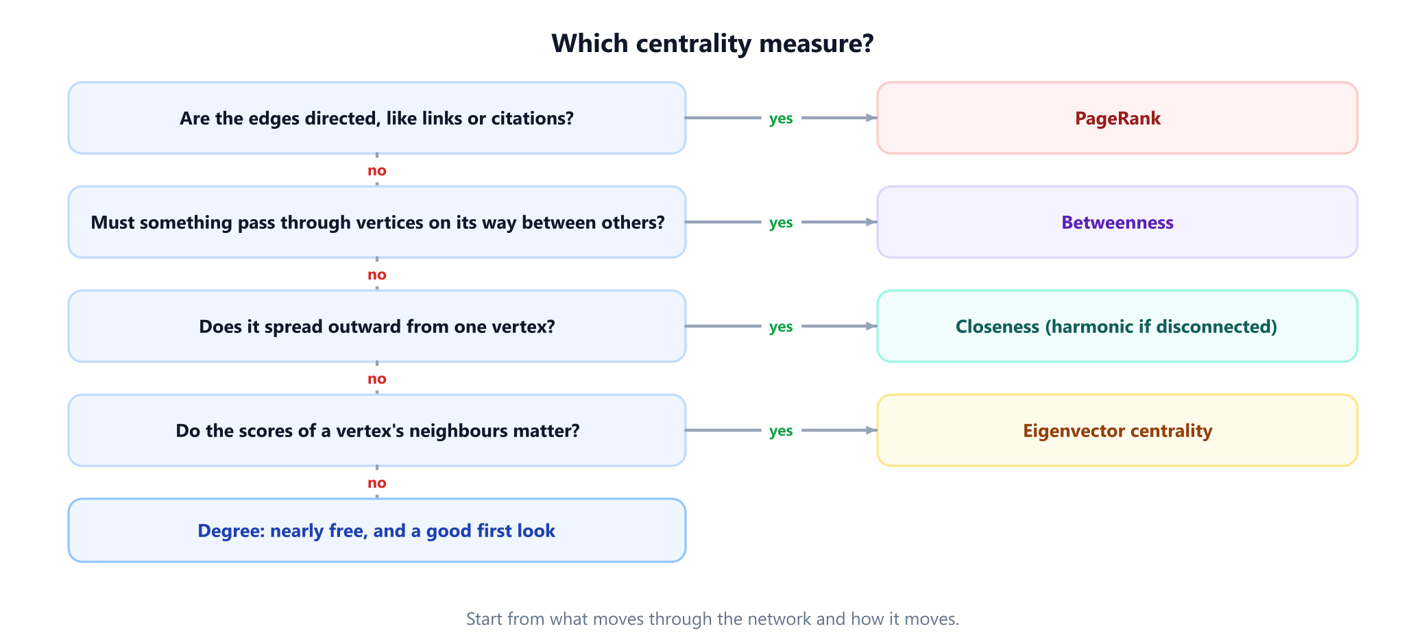
In one sentence: decide what travels through your network and how, then pick the measure that models it. If you only want a starting point, compute degree first, because it is nearly free and the others are best read as corrections to it. The chart below turns that advice into four questions.
2. One company, four winners
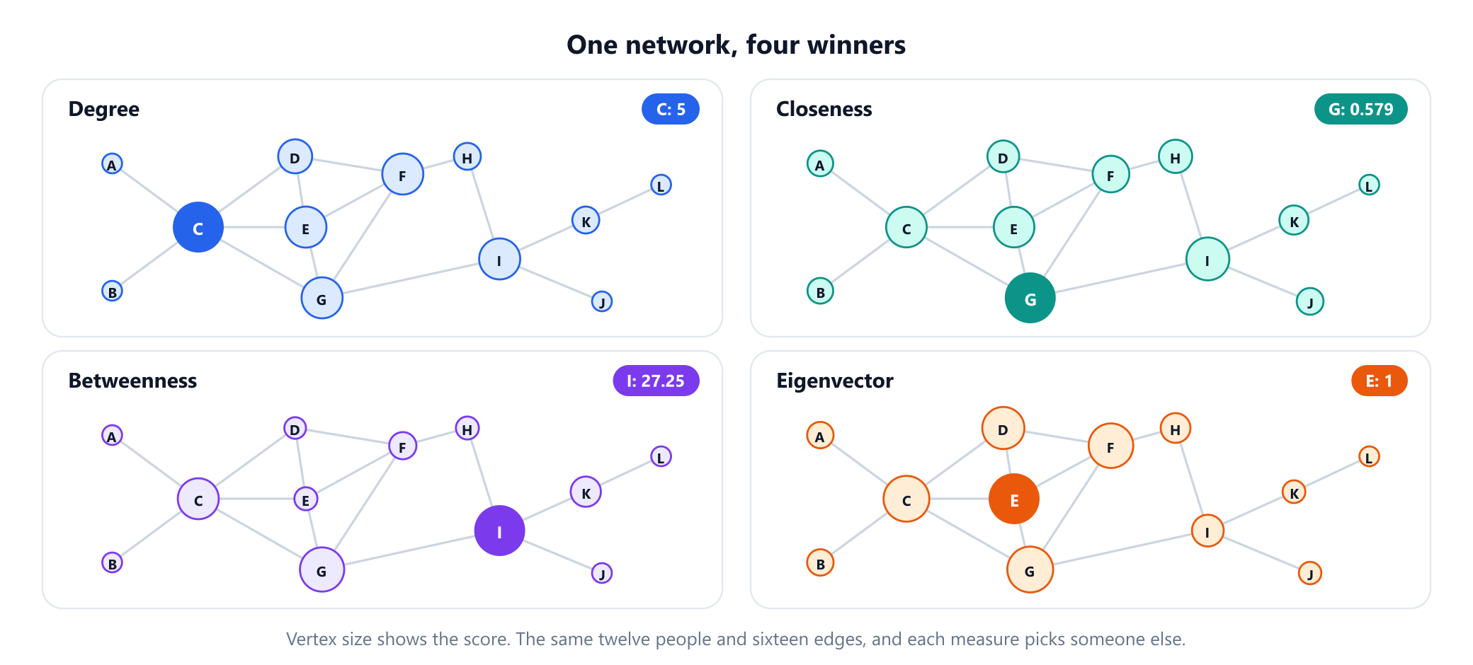
The running example is a company of twelve people, A to L, with an edge between two people who work together directly. It has 16 edges and was found by a computer search for a small network on which degree, closeness, betweenness and eigenvector centrality each pick a different person. That extends the idea of David Krackhardt's "kite" network of 1990, ten people on which degree, closeness and betweenness favour different people.
| Person | Degree | Closeness | Betweenness | Eigenvector |
|---|---|---|---|---|
| A | 1 | 0.344 | 0 | 0.262 |
| B | 1 | 0.344 | 0 | 0.262 |
| C | 5 | 0.500 | 20.33 | 0.921 |
| D | 3 | 0.407 | 1.75 | 0.796 |
| E | 4 | 0.500 | 3.08 | 1.000 |
| F | 4 | 0.458 | 7.08 | 0.879 |
| G | 4 | 0.579 | 23.50 | 0.922 |
| H | 2 | 0.423 | 3.00 | 0.376 |
| I | 4 | 0.524 | 27.25 | 0.444 |
| J | 1 | 0.355 | 0 | 0.126 |
| K | 2 | 0.379 | 10.00 | 0.137 |
| L | 1 | 0.282 | 0 | 0.039 |
All four answers are correct. C has the most contacts, two of whom know nobody else. G can reach the whole company in the fewest total steps. I is the only link between J, K and L and the rest of the company. And E sits in the middle of the tightly knit group. Notice how badly the winners do on each other's measures: E is sixth by betweenness and I is sixth by eigenvector centrality. Sections 3 to 5 explain each column and give the code that produced it.
3. Degree and closeness: contacts and reach
Degree centrality is the number of edges at a vertex, which the guide to vertex degree covers in depth. It only looks one step away, so it costs almost nothing and it misses everything beyond the neighbours. C wins with 5, and on a directed graph it splits into in-degree and out-degree.
Closeness centrality looks at every vertex. For a vertex v in a connected graph, add up the shortest distances from v to all the others, then invert the result so that a higher score means closer: (n - 1) / sum of distances. Distances come from a breadth-first search from each vertex. The program below is saved as people.py, because later programs import it.
from collections import deque

# Who works directly with whom in a company of twelve.
PEOPLE = 'AC BC CD CE CG DE DF EF EG FG FH GI HI IJ IK KL'.split()

def graph(edges):
    adj = {}
    for a, b in edges:
        adj.setdefault(a, []).append(b)
        adj.setdefault(b, []).append(a)
    return adj

def distances(adj, source):
    """Breadth-first search: number of steps from source to everything it can reach."""
    dist, queue = {source: 0}, deque([source])
    while queue:
        v = queue.popleft()
        for w in adj[v]:
            if w not in dist:
                dist[w] = dist[v] + 1
                queue.append(w)
    return dist

def degree(adj):
    return {v: len(adj[v]) for v in adj}

def closeness(adj):
    """(reachable vertices) / (sum of distances to them): misleading if adj is disconnected."""
    result = {}
    for v in adj:
        dist = distances(adj, v)
        result[v] = (len(dist) - 1) / sum(dist.values()) if len(dist) > 1 else 0.0
    return result

def harmonic(adj):
    """Average of 1 / distance over all other vertices; an unreachable vertex adds 0."""
    n = len(adj)
    return {v: sum(1 / d for d in distances(adj, v).values() if d) / (n - 1) for v in adj}

def winner(score):
    return max(sorted(score), key=score.get)

if __name__ == '__main__':
    adj = graph(PEOPLE)
    d, c, h = degree(adj), closeness(adj), harmonic(adj)
    print('most contacts: ', winner(d), d[winner(d)])
    print('closest to all:', winner(c), round(c[winner(c)], 3))
    # Add a pair of contractors who only work with each other.
    split = graph(PEOPLE + ['XY'])
    c2, h2 = closeness(split), harmonic(split)
    print('naive closeness, X:', round(c2['X'], 3), ' G:', round(c2['G'], 3))
    print('harmonic,        X:', round(h2['X'], 3), ' G:', round(h2['G'], 3))
# most contacts:  C 5
# closest to all: G 0.579
# naive closeness, X: 1.0  G: 0.579
# harmonic,        X: 0.077  G: 0.564
G reaches the other eleven people in 19 steps in total, so its closeness is 11 / 19 = 0.579.
The last two lines of output show the standard trap. Closeness assumes that everyone can reach everyone. Add a pair of contractors, X and Y, who only work with each other, and the usual workaround of summing over reachable vertices gives X a perfect score of 1.0, far above G, simply because its tiny component is one step wide. Harmonic centrality fixes this by averaging 1 / distance over all other vertices, so that an unreachable vertex contributes 0. It gives X only 0.077 and leaves G at 0.564. The measure was first proposed by Massimo Marchiori and Vito Latora in 2000, and Paolo Boldi and Sebastiano Vigna's 2014 study of what a centrality measure should satisfy found it the only measure they tested that meets all three of their axioms. Use it whenever a graph may be disconnected; the guide to connected components shows how to check.
4. Betweenness: who the routes pass through
Betweenness centrality asks a different question: if everyone sent one message to everyone else along shortest routes, how many of those messages would pass through v? For each pair s, t not including v, it takes the fraction of shortest s-t paths that go through v, and adds up those fractions. Fractions matter: in a square S, X, T, Y, there are two equally short routes from S to T, so X and Y get half a point each from that pair.
Counted directly, this takes O(V³) time or worse. In 2001 Ulrik Brandes showed how to do it in O(VE) on an unweighted graph, by running one breadth-first search per source and then walking back from the farthest vertex. The key is that the credit each vertex passes up can be worked out from the credit of the vertices below it, instead of being recomputed for each target.
from collections import deque
from people import PEOPLE, graph

def betweenness(adj, sources=None):
    """Brandes' algorithm for an undirected, unweighted graph.

    sources=None uses every vertex and is exact. A list of sources gives an estimate."""
    sources = list(adj) if sources is None else sources
    score = dict.fromkeys(adj, 0.0)
    for s in sources:
        # Phase 1: BFS from s, counting shortest paths (sigma) and recording predecessors.
        order, preds, sigma, dist = [], {v: [] for v in adj}, dict.fromkeys(adj, 0), {s: 0}
        sigma[s] = 1
        queue = deque([s])
        while queue:
            v = queue.popleft()
            order.append(v)
            for w in adj[v]:
                if w not in dist:
                    dist[w] = dist[v] + 1
                    queue.append(w)
                if dist[w] == dist[v] + 1:
                    sigma[w] += sigma[v]
                    preds[w].append(v)
        # Phase 2: walk back from the farthest vertex, handing credit to predecessors.
        delta = dict.fromkeys(adj, 0.0)
        for w in reversed(order):
            for v in preds[w]:
                delta[v] += sigma[v] / sigma[w] * (1 + delta[w])
            if w != s:
                score[w] += delta[w]
    scale = len(adj) / len(sources) / 2          # each pair is seen from both of its ends
    return {v: x * scale for v, x in score.items()}

if __name__ == '__main__':
    b = betweenness(graph(PEOPLE))
    for v in sorted(b, key=b.get, reverse=True)[:5]:
        print(v, round(b[v], 2))
    print(betweenness(graph('SX XT SY YT'.split())))   # two equal routes from S to T
# I 27.25
# G 23.5
# C 20.33
# K 10.0
# F 7.08
# {'S': 0.5, 'X': 0.5, 'T': 0.5, 'Y': 0.5}
Every search counts each pair twice, once from each end, which is why the program divides by 2 on an undirected graph. On a weighted graph, Dijkstra replaces breadth-first search and the time becomes O(VE + V² log V).
I scores 27.25 out of a possible 55, the number of pairs that do not include I, so about half of the shortest routes between other pairs pass through it. Of those 27.25 points, 26 come from pairs involving J, K or L, who have no other way out. I has only four contacts, the same as E, F and G, which is exactly what degree cannot show.
5. Eigenvector centrality: who your contacts are
Degree counts contacts as if they were all equal. Eigenvector centrality says a contact is worth as much as that contact's own score, so a vertex's score is proportional to the sum of its neighbours' scores: x = (1 / λ) A x, with A the adjacency matrix. That makes x an eigenvector of A. On a connected undirected graph, the Perron-Frobenius theorem guarantees exactly one eigenvector with all positive entries, up to scaling, belonging to the largest eigenvalue, and that is the score. Phillip Bonacich made it a standard tool of network analysis in 1972, though John Seeley had used a similar score on sociometric data in 1949.
The standard way to compute it is power iteration: start with equal scores, replace each with the sum of its neighbours, rescale, and repeat.
from people import PEOPLE, graph

def eigenvector(adj, shift=1.0, steps=2000):
    """Power iteration on A + shift * I, scaled so that the top score is 1."""
    x = dict.fromkeys(adj, 1.0)
    for _ in range(steps):
        y = {v: shift * x[v] + sum(x[u] for u in adj[v]) for v in adj}
        top = max(y.values())
        x = {v: y[v] / top for v in y}
    return x

if __name__ == '__main__':
    e = eigenvector(graph(PEOPLE))
    for v in sorted(e, key=e.get, reverse=True)[:4]:
        print(v, round(e[v], 3))
    # Without the shift, a bipartite graph can make the iteration jump forever.
    path = graph('AB BC CD'.split())
    x = {'A': 1.0, 'B': 0.0, 'C': 0.0, 'D': 0.0}
    for step in range(1, 52):
        y = {v: sum(x[u] for u in path[v]) for v in path}
        top = max(y.values())
        x = {v: y[v] / top for v in y}
        if step >= 50:
            print('step', step, {v: round(x[v], 3) for v in sorted(x)})
    print('with the shift', {v: round(s, 3) for v, s in sorted(eigenvector(path).items())})
# E 1.0
# G 0.922
# C 0.921
# F 0.879
# step 50 {'A': 0.618, 'B': 0.0, 'C': 1.0, 'D': 0.0}
# step 51 {'A': 0.0, 'B': 1.0, 'C': 0.0, 'D': 0.618}
# with the shift {'A': 0.618, 'B': 1.0, 'C': 1.0, 'D': 0.618}
E wins even though C has more contacts and G is closer to everyone. The scores of E's four contacts add up to 3.519. G's four add up to only 3.244, because one of them is I, which scores just 0.444 and leads out to the edge of the company.
The output also shows why the code adds shift. On a bipartite graph, A has an eigenvalue of equal size and opposite sign, so plain power iteration may never settle: on a path of four vertices, started from a single vertex, the scores jump between two states forever, with half of them at 0 on each step. Iterating with A + I moves every eigenvalue up by 1, removes the tie and leaves the eigenvectors unchanged. The guide to spectral graph theory covers what the other eigenvalues tell you.
On directed graphs the measure breaks down: a vertex nobody points to scores 0, and so does everything that it alone points to. Leo Katz's measure of 1953 avoids that problem: it counts every walk into a vertex, a walk of length k weighted by α^k. In modern form it reads x = α Aᵀ x + 1, with α below 1 / λ, which amounts to giving every vertex a small amount of free score. PageRank makes one further change.
6. PageRank: following the links
PageRank, published by Sergey Brin and Larry Page in 1998, was designed for the web, where a link from a page is a vote for another page. Katz's measure has a flaw there: a page that links to a thousand others passes its full score to each one. PageRank makes each page split its score among its outgoing links.
The usual picture is a random surfer. At each step the surfer follows a random link from the current page with probability d, the damping factor, and otherwise jumps to a page chosen uniformly at random. A page's rank is the long-run fraction of time spent on it. In the normalised form, where all the ranks add up to 1:
rank(p) = (1 - d) / n + d * sum of rank(q) / outdegree(q), over pages q that link to pThe example is a web of eight pages. Every page can reach every other, so nothing is cut off. Brin and Page reported that they usually set d to 0.85, and the program does the same.
# Eight web pages and the pages each one links to.
WEB = {'A': 'CH', 'B': 'CDEH', 'C': 'A', 'D': 'C', 'E': 'D', 'F': 'BDG', 'G': 'D', 'H': 'AF'}

def pagerank(links, d=0.85, tol=1e-10):
    """Power iteration. A page with no outgoing links shares its rank with every page."""
    pages = sorted(links)
    n = len(pages)
    rank = dict.fromkeys(pages, 1 / n)
    steps = 0
    while True:
        dangling = sum(rank[p] for p in pages if not links[p])
        new = dict.fromkeys(pages, (1 - d) / n + d * dangling / n)
        for p in pages:
            for q in links[p]:
                new[q] += d * rank[p] / len(links[p])
        change = sum(abs(new[p] - rank[p]) for p in pages)
        rank, steps = new, steps + 1
        if change < tol:
            return rank, steps

if __name__ == '__main__':
    rank, steps = pagerank(WEB)
    inlinks = {p: sum(p in out for out in WEB.values()) for p in WEB}
    for p in sorted(rank, key=rank.get, reverse=True):
        print(p, 'in-links', inlinks[p], ' rank', round(rank[p], 3))
    print('iterations', steps, ' total', round(sum(rank.values()), 6))
# A in-links 2  rank 0.293
# C in-links 3  rank 0.247
# H in-links 2  rank 0.152
# D in-links 4  rank 0.111
# F in-links 1  rank 0.084
# B in-links 1  rank 0.042
# G in-links 1  rank 0.042
# E in-links 1  rank 0.028
# iterations 70  total 1.0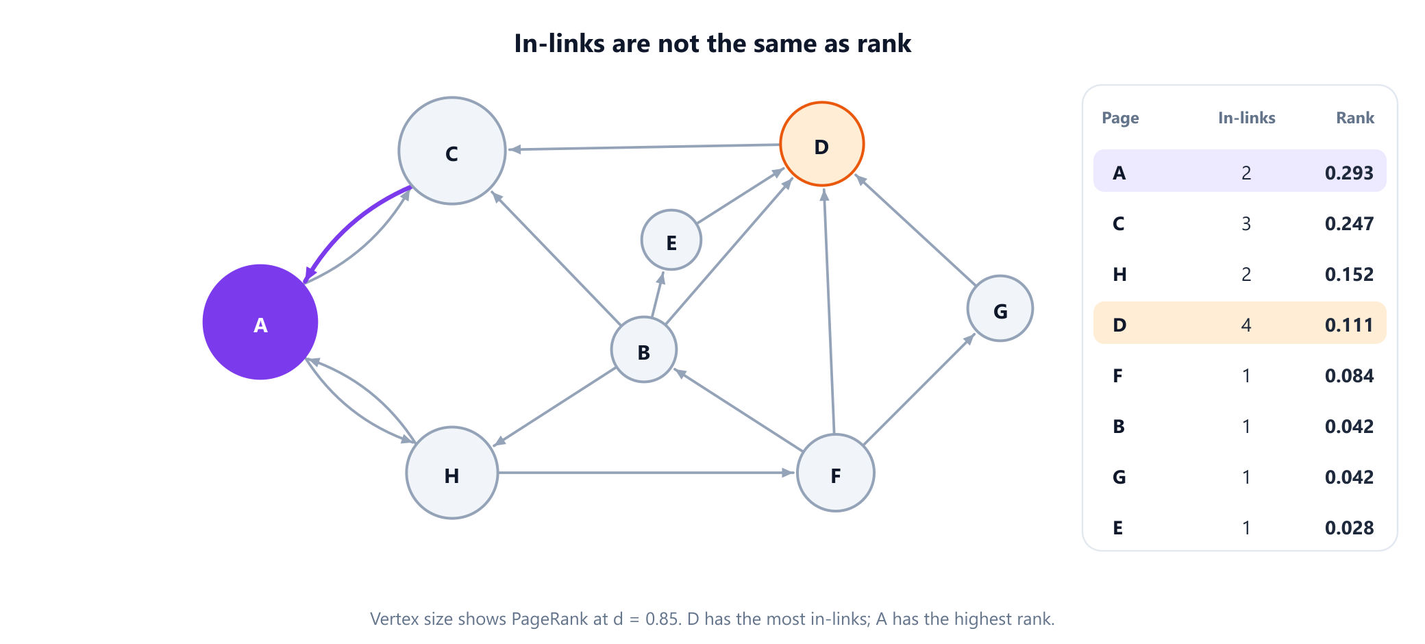
D has the most incoming links, four, but they come from pages with little rank to give, and B and F divide theirs among several links. D then passes all of its rank to C, and C passes all of its rank to A. So A, with only two in-links, finishes first with 0.293, and A and C together hold 54% of the total. On an undirected graph, the picture is much plainer: with d = 1 on a connected non-bipartite graph, PageRank is exactly proportional to degree. PageRank is mainly a measure for directed graphs, and the guide to directed and undirected graphs explains why the distinction matters.
7. Dead ends, closed loops and the damping factor
The damping factor is not decoration. Two kinds of page break the plain "follow a link" process, and the next program breaks the example web in both ways.
from pagerank import WEB, pagerank

def leaky(links, d=0.85, steps=200):
    """The textbook update with no handling of dead ends."""
    n = len(links)
    rank = dict.fromkeys(links, 1 / n)
    for _ in range(steps):
        new = dict.fromkeys(links, (1 - d) / n)
        for p in links:
            for q in links[p]:
                new[q] += d * rank[p] / len(links[p])
        rank = new
    return rank

if __name__ == '__main__':
    dead_end = {**WEB, 'A': ''}                    # A no longer links anywhere
    print('dead end, naive update:   total', round(sum(leaky(dead_end).values()), 3))
    print('dead end, handled:        total', round(sum(pagerank(dead_end)[0].values()), 3))
    closed = {**WEB, 'A': 'C'}                     # A and C now only link to each other
    for d in (0.85, 0.999):
        rank = pagerank(closed, d=d, tol=1e-9)[0]
        print(f'closed loop, d = {d}: A + C hold', round(rank['A'] + rank['C'], 3))
# dead end, naive update:   total 0.403
# dead end, handled:        total 1.0
# closed loop, d = 0.85: A + C hold 0.791
# closed loop, d = 0.999: A + C hold 0.998
A dead end is a page with no outgoing links. The textbook update has nowhere to send its rank, so rank leaks out of the system: with A turned into a dead end, the total falls from 1 to 0.403. The fix, used in the pagerank function above, is to share a dead end's rank among all pages, as if the surfer jumped at random from there.
A closed loop is a group of pages that link only to each other. Once the surfer enters, only the random jump gets it out. Make A link only to C and the pair holds 79.1% of all rank at d = 0.85, and 99.8% at d = 0.999. The smaller d is, the less a loop can absorb.
The price of a large d is speed. The change in the ranks shrinks by at least a factor of d at every step, which matches the result of Taher Haveliwala and Sepandar Kamvar that the second eigenvalue of the PageRank matrix is at most d in absolute value. The next program measures that on a web of 1,000 pages grouped into 20 sites.
import random

def web(sites, size, rnd):
    """Pages link mostly inside their own site; about one page in ten links to another site."""
    links = {}
    for s in range(sites):
        for i in range(size):
            out = {s * size + rnd.randrange(size) for _ in range(5)}
            if rnd.random() < 0.1:
                out.add(rnd.randrange(sites * size))
            links[s * size + i] = sorted(out - {s * size + i})
    return links

def steps_needed(links, d, tol=1e-6):
    n = len(links)
    rank, step = dict.fromkeys(links, 1 / n), 0
    while True:
        lost = sum(rank[p] for p in links if not links[p])
        new = dict.fromkeys(links, (1 - d) / n + d * lost / n)
        for p in links:
            for q in links[p]:
                new[q] += d * rank[p] / len(links[p])
        change = sum(abs(new[p] - rank[p]) for p in links)
        rank, step = new, step + 1
        if change < tol:
            return step

if __name__ == '__main__':
    links = web(20, 50, random.Random(5))
    for d in (0.5, 0.85, 0.95, 0.99):
        print('d =', d, ' iterations:', steps_needed(links, d))
# d = 0.5  iterations: 13
# d = 0.85  iterations: 53
# d = 0.95  iterations: 149
# d = 0.99  iterations: 607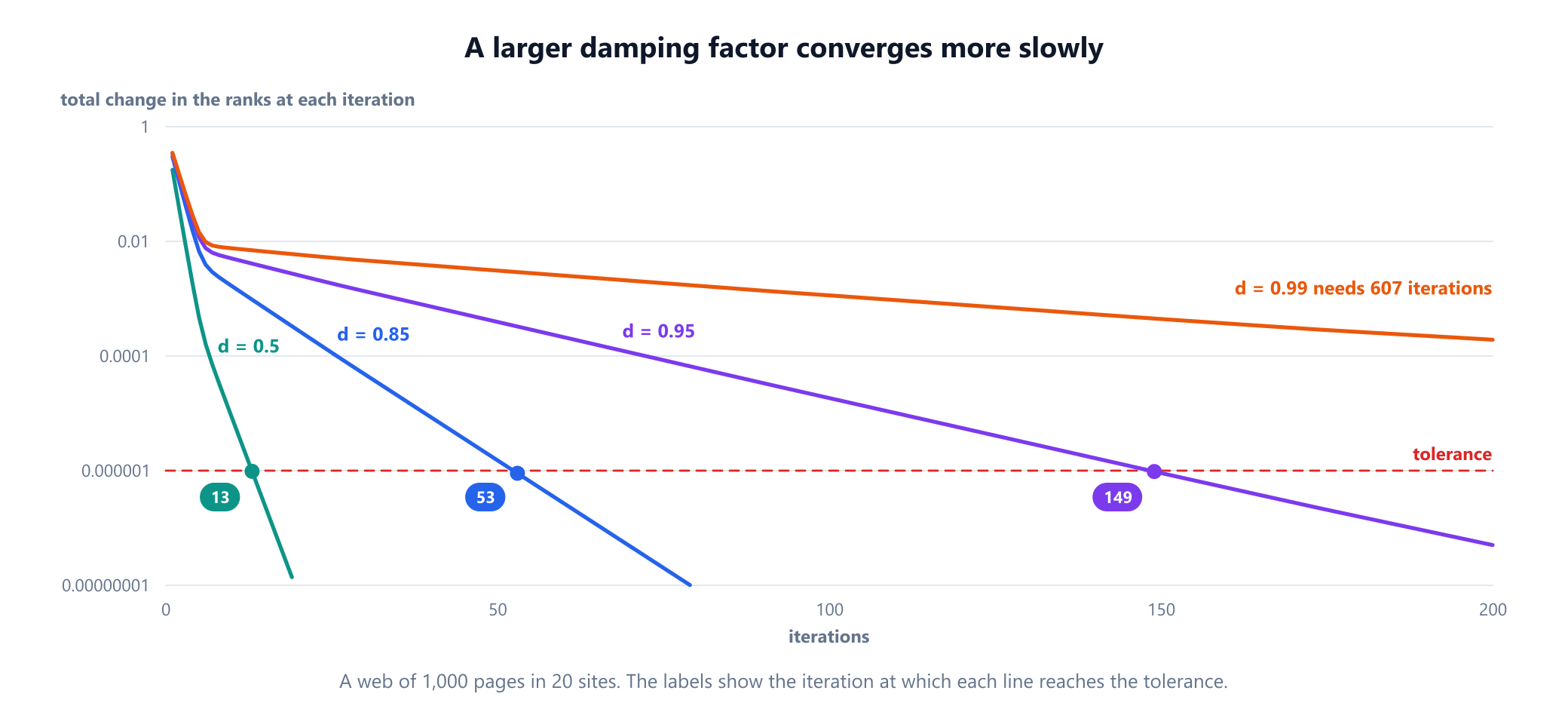
8. Do the measures agree?
If the measures usually named the same vertices, you could always use the cheapest. The next program builds three kinds of network with 400 vertices each, then asks how many of the top 20 vertices by betweenness are also in the top 20 by each of the other measures.
import random
from people import degree, closeness
from brandes import betweenness
from eigen import eigenvector

def link(adj, a, b):
    if a != b and b not in adj[a]:
        adj[a].append(b)
        adj[b].append(a)

def hubs(n, m, rnd):
    """Preferential attachment: newcomers favour vertices that already have many edges."""
    adj = {v: [] for v in range(n)}
    pool = list(range(m))
    for v in range(m, n):
        for t in set(rnd.choice(pool) for _ in range(m)):
            link(adj, v, t)
            pool += [v, t]
    return adj

def two_groups(n, rnd):
    """Two dense halves joined by only six edges."""
    adj = {v: [] for v in range(n)}
    half = n // 2
    for a in range(n):
        for b in range(a + 1, n):
            if (a < half) == (b < half) and rnd.random() < 0.05:
                link(adj, a, b)
    for _ in range(6):
        link(adj, rnd.randrange(half), rnd.randrange(half, n))
    return adj

def ring(n, rnd):
    """Each vertex linked to its 3 nearest neighbours each way; 5% of edges rewired."""
    adj = {v: [] for v in range(n)}
    for v in range(n):
        for k in (1, 2, 3):
            link(adj, v, rnd.randrange(n) if rnd.random() < 0.05 else (v + k) % n)
    return adj

def top(score, k=20):
    return set(sorted(score, key=lambda v: (-score[v], v))[:k])

if __name__ == '__main__':
    rnd = random.Random(11)
    print('top 20 by betweenness also in the top 20 by:  degree, closeness, eigenvector')
    for name, adj in (('hubs', hubs(400, 2, rnd)), ('two groups', two_groups(400, rnd)), ('ring', ring(400, rnd))):
        b = top(betweenness(adj))
        print(f'{name:11}', len(b & top(degree(adj))), len(b & top(closeness(adj))), len(b & top(eigenvector(adj, steps=4000))))
# top 20 by betweenness also in the top 20 by:  degree, closeness, eigenvector
# hubs        18 13 14
# two groups  8 17 4
# ring        6 9 1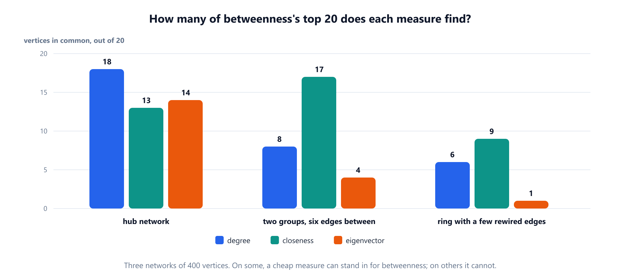
On the hub network, where a few vertices collect most edges, degree finds 18 of the 20, so paying for betweenness buys little. On the two groups joined by six edges, degree finds only 8 and eigenvector centrality only 4, because all 20 of its top vertices lie in the same group: it concentrates on one half and cannot see the other. On the ring, where structure is mostly local, the measures largely pick different vertices. Before relying on a cheap substitute, test it on a sample of your own network.
9. Large graphs: estimating betweenness
Exact betweenness needs one search per vertex, which is out of reach on graphs with hundreds of millions of vertices. The standard shortcut, studied by Brandes and Christian Pich in 2007, is to run the search from a random sample of source vertices and scale the result up. The sources argument of the program in section 4 already does that.
import random
from brandes import betweenness
from agree import hubs, top

if __name__ == '__main__':
    rnd = random.Random(3)
    adj = hubs(1000, 3, rnd)
    exact = betweenness(adj)
    best = top(exact, 10)
    print('sources  work  top 10 found  mean error of the top 10   (average of 10 runs)')
    for k in (10, 50, 100, 250, 500):
        found = error = 0
        for _ in range(10):
            estimate = betweenness(adj, rnd.sample(sorted(adj), k))
            found += len(best & top(estimate, 10))
            error += sum(abs(estimate[v] - exact[v]) / exact[v] for v in best) / 10
        print(f'{k:7} {k / 10:4.0f}% {found / 10:13.1f} {error / 10:12.1%}')
# sources  work  top 10 found  mean error of the top 10   (average of 10 runs)
#      10    1%           6.2        36.8%
#      50    5%           8.1        17.3%
#     100   10%           9.4        13.4%
#     250   25%           9.1         8.6%
#     500   50%           9.4         4.0%
On this network of 1,000 vertices, 10% of the work finds on average 9.4 of the true top 10 vertices, with a typical error of about 13% in their scores. Sampling is good at finding the top of the list, and much less exact about the scores themselves. A sample of 1% is too small, finding only 6.2. Degree, by contrast, stays cheap at any size, and eigenvector centrality and PageRank need only a limited number of passes over the edges, which is why they scale to web-sized graphs.
10. Where these measures are used
- Web search. PageRank was a central part of the first Google search engine, combined with other signals such as the text of pages and links.
- Biology. Hawoong Jeong and colleagues reported in 2001 that in the protein network of yeast, highly connected proteins are more likely to be essential for survival. The guide to graph theory in biology looks at hubs and bottlenecks.
- Community detection. Michelle Girvan and Mark Newman's method of 2002 repeatedly removes the edge with the highest betweenness and recomputes betweenness after each removal, since edges between groups carry the most routes.
- Security. Betweenness points at the hosts that the most attack paths go through, which is where a single fix helps most; see graph theory in cybersecurity.
- Machine learning. Centrality scores are common input features for vertices, and graph neural networks learn related quantities from data.
11. A short history
Centrality began in the study of small groups. Alex Bavelas introduced the idea in 1948, and experiments in his Group Networks Laboratory at MIT, reported in his 1950 paper, linked it to how well small groups solved problems. Gert Sabidussi gave a mathematical treatment of closeness in 1966. Leo Katz's status index appeared in 1953, and Phillip Bonacich's eigenvector measure in 1972. Jac Anthonisse, in an unpublished report of 1971, and Linton Freeman, in 1977, defined betweenness independently, and Freeman's 1979 paper organised degree, closeness and betweenness into the framework still taught today. PageRank followed in 1998, and Massimo Franceschet's 2011 history traces its ideas back through bibliometrics, sociometry and econometrics, as far as Wassily Leontief's input-output model of 1941 and John Seeley's sociometric index of 1949. Brandes' algorithm of 2001 made betweenness practical on large networks.
12. Common mistakes
| Mistake | Why it is wrong | Fix |
|---|---|---|
| Asking for "the" most important vertex | On the example, four measures name four people | Decide what travels through the network first |
| Treating in-links as rank | D has the most in-links and ranks fourth | Use PageRank when the source of a link matters |
| Closeness on a disconnected graph | A pair of isolated contractors scored 1.0 | Use harmonic centrality |
| Forgetting to halve undirected betweenness | Each pair is counted from both ends | Divide by 2 |
| Using tie strength as distance | Shortest-path measures treat a strong tie as a long one | Convert weights to distances first, for example 1 / w |
| Comparing raw scores between graphs | Betweenness grows with the size of the graph | Normalise, or compare ranks |
| Plain power iteration on a bipartite graph | The scores can oscillate forever | Iterate with A + I |
| Ignoring dead ends in PageRank | The total rank drained to 0.403 | Share a dead end's rank among all pages |
13. Glossary
| Term | Meaning |
|---|---|
| Centrality | A score for how important a vertex is, under a stated definition |
| Degree centrality | The number of edges at a vertex |
| Closeness centrality | (n - 1) divided by the sum of distances to all other vertices |
| Harmonic centrality | The average of 1 / distance over all other vertices |
| Betweenness centrality | The sum, over pairs, of the fraction of shortest paths through a vertex |
| Eigenvector centrality | A score proportional to the sum of the neighbours' scores |
| Katz centrality | Eigenvector centrality with a small constant added for every vertex |
| PageRank | The long-run share of time a random surfer spends on a page |
| Damping factor | The probability d that the surfer follows a link rather than jumps |
| Dead end | A page with no outgoing links |
| Power iteration | Repeatedly multiplying by a matrix and rescaling, to find its main eigenvector |
| Brandes' algorithm | Exact betweenness in O(VE) on an unweighted graph |
14. Frequently asked questions
What is centrality in graph theory?
Centrality is any score that says how important a vertex is within a graph. Different definitions capture different kinds of importance: the number of direct connections, the distance to everyone else, the share of shortest routes passing through the vertex, or the importance of its neighbours. On the same graph these definitions can name different vertices.
What is the difference between degree, closeness and betweenness centrality?
Degree counts a vertex's direct connections. Closeness measures how few steps it takes to reach all other vertices. Betweenness measures how many of the shortest routes between other pairs pass through the vertex. A person can have few contacts and still score highest on betweenness by being the only link between two groups.
What is the difference between PageRank and eigenvector centrality?
Both give a vertex a score based on the scores of the vertices connected to it. PageRank is designed for directed graphs: each page splits its rank among its outgoing links, and a damping factor adds a random jump, so pages with no in-links and closed groups of pages cannot break it. Eigenvector centrality is mainly used on connected undirected graphs.
Which centrality measure should I use?
It depends on what moves through the network. Use PageRank for directed links or citations, betweenness when something must pass through vertices on its way between others, closeness or harmonic centrality when something spreads outward from one place, eigenvector centrality when the quality of neighbours matters, and degree when you want a fast first answer.
How is betweenness centrality computed?
Brandes' algorithm runs a breadth-first search from every vertex, counting shortest paths, then walks back from the farthest vertex and passes credit to predecessors. It takes O(VE) time on an unweighted graph. On very large graphs, running it from a random sample of sources and scaling up gives a good estimate of the top vertices.
What is the damping factor in PageRank?
The damping factor d is the probability that the random surfer follows a link rather than jumping to a random page. Brin and Page reported usually setting it to 0.85. A larger d follows the link structure more closely but needs more iterations and lets closed groups of pages absorb more rank.
15. References
The algorithms, results and attributions above come from these sources, listed in chronological order.
- Bavelas, A. (1948). "A Mathematical Model for Group Structures." Human Organization 7(3), 16 to 30.
- Seeley, J. R. (1949). "The Net of Reciprocal Influence: A Problem in Treating Sociometric Data." Canadian Journal of Psychology 3(4), 234 to 240.
- Bavelas, A. (1950). "Communication Patterns in Task-Oriented Groups." Journal of the Acoustical Society of America 22(6), 725 to 730.
- Katz, L. (1953). "A New Status Index Derived from Sociometric Analysis." Psychometrika 18(1), 39 to 43.
- Sabidussi, G. (1966). "The Centrality Index of a Graph." Psychometrika 31(4), 581 to 603.
- Anthonisse, J. M. (1971). "The Rush in a Directed Graph." Report BN 9/71, Stichting Mathematisch Centrum, Amsterdam.
- Bonacich, P. (1972). "Factoring and Weighting Approaches to Status Scores and Clique Identification." Journal of Mathematical Sociology 2(1), 113 to 120.
- Freeman, L. C. (1977). "A Set of Measures of Centrality Based on Betweenness." Sociometry 40(1), 35 to 41.
- Freeman, L. C. (1979). "Centrality in Social Networks: Conceptual Clarification." Social Networks 1(3), 215 to 239.
- Krackhardt, D. (1990). "Assessing the Political Landscape: Structure, Cognition, and Power in Organizations." Administrative Science Quarterly 35(2), 342 to 369.
- Brin, S. and Page, L. (1998). "The Anatomy of a Large-Scale Hypertextual Web Search Engine." Computer Networks and ISDN Systems 30(1 to 7), 107 to 117.
- Marchiori, M. and Latora, V. (2000). "Harmony in the Small-World." Physica A 285(3 to 4), 539 to 546.
- Brandes, U. (2001). "A Faster Algorithm for Betweenness Centrality." Journal of Mathematical Sociology 25(2), 163 to 177.
- Jeong, H., Mason, S. P., Barabási, A.-L. and Oltvai, Z. N. (2001). "Lethality and Centrality in Protein Networks." Nature 411, 41 to 42.
- Girvan, M. and Newman, M. E. J. (2002). "Community Structure in Social and Biological Networks." Proceedings of the National Academy of Sciences 99(12), 7821 to 7826.
- Haveliwala, T. H. and Kamvar, S. D. (2003). "The Second Eigenvalue of the Google Matrix." Technical Report, Stanford University.
- Brandes, U. and Pich, C. (2007). "Centrality Estimation in Large Networks." International Journal of Bifurcation and Chaos 17(7), 2303 to 2318.
- Franceschet, M. (2011). "PageRank: Standing on the Shoulders of Giants." Communications of the ACM 54(6), 92 to 101.
- Boldi, P. and Vigna, S. (2014). "Axioms for Centrality." Internet Mathematics 10(3 to 4), 222 to 262.
See the search behind the scores
Closeness and betweenness both start with a breadth-first search from every vertex. Draw a small network in the visualizer and run the search from two different vertices to see why one reaches everyone sooner.
Open the visualizer