
Table of Contents
- 1. The degree of a vertex
- 2. The handshaking lemma
- 3. Computing degrees from a stored graph
- 4. Puzzles the lemma settles at once
- 5. Degree sequences: which lists can be graphs?
- 6. What a large minimum degree guarantees
- 7. What the maximum degree bounds
- 8. Degeneracy and k-cores
- 9. The friendship paradox
- 10. Degree distributions in real networks
- 11. Directed graphs: in-degree and out-degree
- 12. Common mistakes
- 13. Glossary
- 14. Frequently asked questions
- 15. References
1. The degree of a vertex
The degree of a vertex is the number of edges that meet it. In a simple graph that is the same as the number of its neighbours. It is the most local number a graph has: you can read it off one vertex without looking at anything else. Yet a surprising amount of global structure is decided by degrees alone, and that is what this article is about.
The notation is short. deg(v) is the degree of v, δ(G) is the minimum degree over all vertices and Δ(G) the maximum degree. A vertex of degree 0 is isolated, a vertex of degree 1 is a leaf or pendant vertex, and a graph in which every vertex has the same degree r is r-regular. The basic vocabulary, including why a loop adds 2 to a degree, is set out in the guide to vertices and edges; this article takes it as the starting point and asks what degrees can tell you.
One small friendship network carries the whole article. Eight people, A to H, and twelve friendships:
E = {AB, AC, AD, BC, BD, CD, AE, DE, AF, EF, FG, AH}       12 edges

deg:   A 6   B 3   C 3   D 4   E 3   F 3   G 1   H 1
δ = 1 (G and H)      Δ = 6 (A)      average degree = 24 / 8 = 3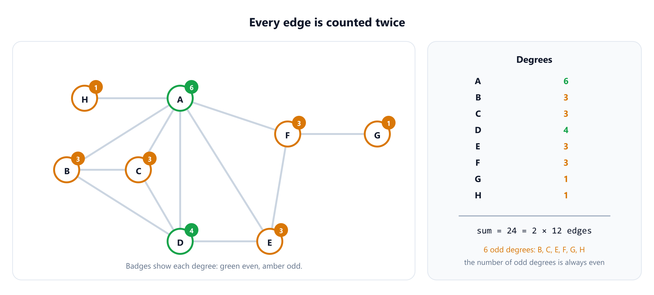
2. The handshaking lemma
Add up the degrees of the example and you get 24, exactly twice its 12 edges. That is not a coincidence of this graph.
Handshaking lemma. In every graph, the sum of the degrees of all vertices equals twice the number of edges: ∑ deg(v) = 2m.
The proof is a double count. Count the pairs (vertex, edge end at that vertex). Counting by vertices gives the sum of the degrees. Counting by edges gives 2 for every edge, because every edge has exactly two ends, and that includes a loop, whose two ends sit on the same vertex. Both counts describe the same set of pairs, so they are equal. The observation goes back to Euler's 1736 paper on the bridges of Königsberg, where it appears in the language of bridges and land regions; the name "handshaking lemma" is modern, from the picture of a party where every handshake involves two hands.
The lemma's most useful consequence is immediate. The sum of all degrees is even, so the odd degrees must come in pairs:
Every graph has an even number of vertices of odd degree.
In the example the odd-degree vertices are B, C, E, F, G and H: six of them, an even number, as promised.
3. Computing degrees from a stored graph
How cheaply you can read a degree depends on how the graph is stored, the trade-off covered in graph representation. With an adjacency list the degree of v is the length of its list, available in O(1) if the length is stored. With an adjacency matrix it is the sum of row v, which costs O(n). With a bare edge list you have to scan all m edges, so the usual move is to compute every degree in one pass and keep the result. The program below does that, checks the handshaking lemma, and also computes the two averages that section 9 is built on.
from collections import Counter

edges = ['AB', 'AC', 'AD', 'BC', 'BD', 'CD', 'AE', 'DE', 'AF', 'EF', 'FG', 'AH']
adj = {v: set() for v in 'ABCDEFGH'}
for u, v in edges:
    adj[u].add(v)
    adj[v].add(u)

deg = {v: len(adj[v]) for v in adj}
print(deg)
# {'A': 6, 'B': 3, 'C': 3, 'D': 4, 'E': 3, 'F': 3, 'G': 1, 'H': 1}

print(sum(deg.values()), 2 * len(edges))     # the handshake lemma
# 24 24
print(sorted(v for v in deg if deg[v] % 2))   # always an even number of them
# ['B', 'C', 'E', 'F', 'G', 'H']

# The friendship paradox: average degree versus the average degree of a friend.
mean_degree = sum(deg.values()) / len(deg)
mean_friend = sum(deg[v] ** 2 for v in deg) / sum(deg.values())
print(mean_degree, mean_friend)
# 3.0 3.75

# How many people have fewer friends than their friends have, on average?
fewer = [v for v in adj if deg[v] < sum(deg[w] for w in adj[v]) / deg[v]]
print(sorted(fewer))
# ['B', 'C', 'E', 'F', 'G', 'H']
print(Counter(deg.values()).most_common(1))  # some degree always repeats
# [(3, 4)]
Two lines of the output are worth noticing now. The handshaking check prints 24 24. And the last line reports that the degree 3 occurs four times. Some degree always repeats, for a reason section 4 explains.
4. Puzzles the lemma settles at once
The handshaking lemma turns several questions that sound like they need a search into one line of arithmetic.
- Can seven people each shake hands with exactly three others? No. That would need a degree sum of
7 × 3 = 21, which is odd, but every degree sum is twice a whole number of handshakes. - Is there a 3-regular graph on 9 vertices? No, for the same reason. An
r-regular graph onnvertices hasnr / 2edges, so whenris odd,nmust be even. - How many edges does a graph with 10 vertices and average degree 3 have? Exactly 15, because the average degree is
2m / n. - Can a walk use every edge exactly once and start and end at different places, with only one vertex of odd degree? The question never arises: a graph cannot have exactly one odd vertex. Euler's criterion asks for zero or two of them, as the guide to Eulerian paths explains, and the lemma rules out every odd count.
A second classic uses the pigeonhole principle instead:
In every simple graph with at least two vertices, some two vertices have the same degree.
With n vertices the possible degrees are 0, 1, …, n − 1, which is n values for n vertices, so all different would mean every value is used once. But 0 and n − 1 cannot both occur: a vertex of degree n − 1 is adjacent to everyone, so nobody has degree 0. That leaves at most n − 1 usable values for n vertices, and two must share one. In everyday terms: at any party, two people have the same number of friends there. The statement needs the graph to be simple; with parallel edges it fails. It was checked by brute force over every simple graph on up to seven vertices.
5. Degree sequences: which lists can be graphs?
List the degrees from largest to smallest and you get the degree sequence, (6, 4, 3, 3, 3, 3, 1, 1) for the example. A sequence that some simple graph actually has is called graphic. An even sum is necessary, by the handshaking lemma, but far from sufficient: (4, 4, 4, 1, 1) has an even sum and no graph. Three vertices of degree 4 among five would each be adjacent to all the others, which would give the last two vertices degree at least 3.
Two classical tests decide the question exactly. The guide to vertices and edges traces both by hand; here they are as code. The Havel–Hakimi method, from Havel (1955) and Hakimi (1962), repeatedly joins the vertex of largest remaining degree to the next ones in line, and either builds a graph or gets stuck. The Erdős–Gallai theorem of 1960 is a closed-form test: a non-increasing sequence with an even sum is graphic exactly when, for every k, the k largest degrees sum to at most k(k − 1) plus the sum of min(di, k) over the rest.
import heapq

def havel_hakimi(seq):
    """Return the edges of a simple graph with these degrees, or None if none exists."""
    if sum(seq) % 2:
        return None                           # an odd total breaks the handshake lemma
    heap = [(-d, i) for i, d in enumerate(seq) if d > 0]
    heapq.heapify(heap)
    edges = []
    while heap:
        d, v = heapq.heappop(heap)
        d = -d
        if d > len(heap):
            return None                       # not enough other vertices left to join
        taken = [heapq.heappop(heap) for _ in range(d)]
        for dw, w in taken:                   # join v to the d vertices of largest degree
            edges.append((v, w))
            if dw + 1 < 0:
                heapq.heappush(heap, (dw + 1, w))
    return edges

def erdos_gallai(seq):
    """True exactly when the sequence is graphic (Erdős and Gallai, 1960)."""
    d = sorted(seq, reverse=True)
    if sum(d) % 2:
        return False
    for k in range(1, len(d) + 1):
        if sum(d[:k]) > k * (k - 1) + sum(min(x, k) for x in d[k:]):
            return False
    return True

print(len(havel_hakimi([6, 4, 3, 3, 3, 3, 1, 1])))
# 12
print(havel_hakimi([4, 4, 4, 1, 1]), erdos_gallai([4, 4, 4, 1, 1]))
# None False
print(havel_hakimi([3, 3, 3, 3, 3]), erdos_gallai([3, 3, 3, 3, 3]))
# None False
For (4, 4, 4, 1, 1) the Erdős–Gallai inequality fails at k = 3: the three largest degrees sum to 12, but the bound is 3 × 2 + 1 + 1 = 8. Both functions were checked against brute force on every one of the 2,353 non-increasing sequences of length n ≤ 7 with entries at most n − 1, and the Havel–Hakimi function was also checked to return a genuine simple graph with exactly the requested degrees. A graphic sequence usually has many different realisations, so a degree sequence describes a family of graphs, not one graph.
6. What a large minimum degree guarantees
Forcing every vertex to have many neighbours forces structure. The arguments behind the first three facts are all variations on one idea: walk as far as you can and look at where the last vertex's neighbours are.
δ ≥ 2forces a cycle. Take a longest path. Its last vertex has at least two neighbours, and all of them lie on the path, or the path could be extended. One of them is not its predecessor, and that edge closes a cycle.δ ≥ kforces a path with at leastkedges. The same longest path must contain allδneighbours of its last vertex, so it has at leastδ + 1vertices.δ ≥ (n − 1) / 2forces the graph to be connected. Two vertices in different components would each need at least(n − 1) / 2neighbours inside their own components, which together would hold more thannvertices.
The most famous result of this kind is about Hamiltonian cycles, cycles that pass through every vertex once. Deciding whether one exists is NP-complete in general, but a large minimum degree settles it.
Dirac's theorem (1952). Every simple graph withn ≥ 3vertices and minimum degree at leastn / 2has a Hamiltonian cycle.
Ore strengthened it in 1960: it is enough that every two non-adjacent vertices have degrees adding up to at least n. The threshold n / 2 cannot be lowered. The complete bipartite graph K2,3 has five vertices and minimum degree 2, just below 5 / 2, and has no Hamiltonian cycle, because a cycle through all five vertices would have to alternate between the two sides, and the sides have different sizes.
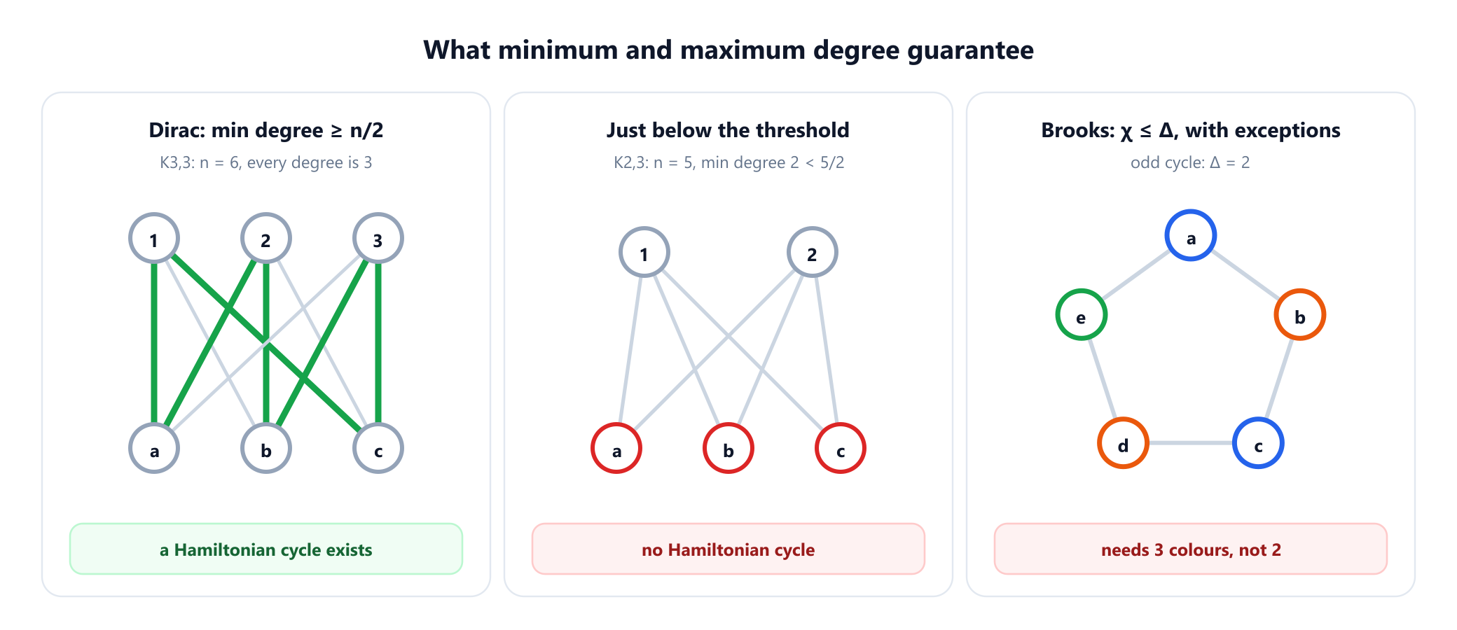
The example network has δ = 1, far below 8 / 2, and it has no Hamiltonian cycle: a cycle can never pass through a leaf such as G, which has only one edge. Dirac's condition is sufficient, not necessary, so failing it proves nothing on its own; here the leaves are the real reason.
7. What the maximum degree bounds
The maximum degree controls colouring. Colour the vertices one at a time in any order, giving each the smallest colour not used by its already coloured neighbours. A vertex has at most Δ neighbours, so at most Δ colours are blocked and one of the first Δ + 1 is always free.
Every graph can be properly coloured with at most Δ + 1 colours, and the greedy algorithm achieves it in any vertex order.
Brooks proved in 1941 that one colour fewer suffices with exactly two kinds of exception: a connected graph needs Δ + 1 colours only if it is a complete graph or an odd cycle. An odd cycle has Δ = 2 and needs 3 colours, and Kn has Δ = n − 1 and needs n. For edge colouring the answer is even tighter: Vizing showed in 1964 that every simple graph can have its edges coloured with Δ or Δ + 1 colours.
In the example Δ = 6, so greedy colouring is guaranteed to use at most 7 colours and Brooks' theorem lowers the bound to 6. The truth is 4, because the example contains the complete graph on A, B, C and D, which needs 4, and 4 are enough. The maximum degree is a crude bound when one vertex is far busier than the rest. Welsh and Powell's 1967 heuristic, which colours the vertices in order of decreasing degree, is one response; the next section gives a sharper one.
8. Degeneracy and k-cores
The hub A inflates Δ without making the graph hard to colour. A better measure looks at how sparse the graph is everywhere, not at its single busiest vertex. Repeatedly delete a vertex of smallest remaining degree. The largest degree you ever had to delete at is the degeneracy of the graph. Equivalently, the k-core is the largest subgraph in which every vertex has at least k neighbours inside it, a notion introduced by Seidman in 1983, and the degeneracy is the largest k with a non-empty k-core.
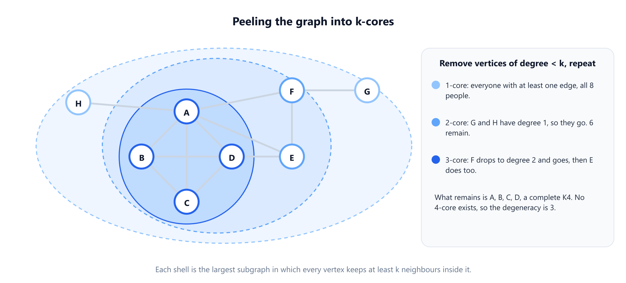
The peeling runs in linear time if vertices are kept in buckets by current degree. Matula and Beck gave such a linear-time smallest-last ordering in 1983, and Batagelj and Zaveršnik's bucket algorithm computes every vertex's core number in O(m):
def core_numbers(adj):
    """Core number of every vertex: peel off a vertex of smallest remaining degree, repeatedly."""
    deg = {v: len(adj[v]) for v in adj}
    buckets = [set() for _ in range(max(deg.values(), default=0) + 1)]
    for v, d in deg.items():
        buckets[d].add(v)
    core, k = {}, 0
    for _ in range(len(adj)):
        d = next(i for i, b in enumerate(buckets) if b)   # smallest non-empty bucket
        k = max(k, d)                         # the core number never goes back down
        v = buckets[d].pop()
        core[v] = k
        for w in adj[v]:
            if w not in core:                 # w loses a neighbour: move it down one bucket
                buckets[deg[w]].remove(w)
                deg[w] -= 1
                buckets[deg[w]].add(w)
    return core

edges = ['AB', 'AC', 'AD', 'BC', 'BD', 'CD', 'AE', 'DE', 'AF', 'EF', 'FG', 'AH']
adj = {v: set() for v in 'ABCDEFGH'}
for u, v in edges:
    adj[u].add(v)
    adj[v].add(u)

core = core_numbers(adj)
print(dict(sorted(core.items())))
# {'A': 3, 'B': 3, 'C': 3, 'D': 3, 'E': 2, 'F': 2, 'G': 1, 'H': 1}
print(max(core.values()))                     # the degeneracy of the graph
# 3
The example's degeneracy is 3, far below its Δ of 6. That matters for colouring, because colouring greedily in the reverse of the peeling order gives every vertex at most degeneracy already coloured neighbours, so it uses at most degeneracy + 1 colours: 4 here, which is optimal. Degeneracy also bounds the work of clique enumeration, where processing vertices in degeneracy order is the standard speed-up, and k-cores are a common first look at large networks: the inner cores are the densely knit centre, the outer shells the periphery.
See degree drive the colouring
Build the example network and run Welsh-Powell, which colours vertices in order of decreasing degree. Then compare the colours it uses with the bound of maximum degree plus one.
Open the graph colouring visualizer9. The friendship paradox
In 1991 the sociologist Scott Feld pointed out something that sounds like an insult: on average, your friends have more friends than you do. It is not a fact about people but about degrees, and the program in section 3 already computed it for the example. The average degree is 3, but the average degree of a friend is 3.75.
The reason is a sampling bias. When you average over people, everyone counts once. When you average over friends, you go through every friendship and look at the person at the other end, so a person with d friends is counted d times. Popular people are over-represented in other people's friend lists precisely because they are popular. In formulas, the average degree is ∑ d / n, while the average degree of a friend is ∑ d² / ∑ d, and the Cauchy–Schwarz inequality shows the second is never smaller than the first, with equality only when every vertex has the same degree.
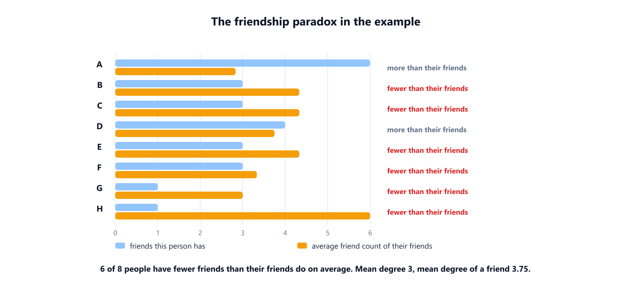
The figure shows a related, person-by-person version: six of the eight people have fewer friends than their own friends have on average, and only A and D come out ahead. The extreme case is a star: in a star with nine leaves the average degree is 1.8 but the average degree of a friend is 5, and every leaf has fewer friends than its one friend. Be careful with the person-by-person version, though. The inequality above is about averages and guarantees nothing about how many individuals fall below. In real networks the effect is strong all the same: in Ugander and colleagues' 2011 study of the Facebook graph, 92.7% of users had fewer friends than the average friend count of their friends.
The paradox has practical uses. A friend of a random person is a better-than-random way to find a well-connected one, which is why sampling friends of random people has been proposed as a way to catch an epidemic early, and why vaccinating acquaintances can protect more people than vaccinating at random.
10. Degree distributions in real networks
For a large network the list of degrees is too long to read, so it is summarised by the degree distribution: the fraction of vertices with degree k, for each k. Its shape says a great deal about how the network was formed.
- Random graphs in the Erdős–Rényi model, where every pair is joined independently, have degrees tightly concentrated around the average, with almost no vertex far from it.
- Many real networks look very different: most vertices have small degree, and a few hubs have enormous degree. Barabási and Albert proposed in 1999 that preferential attachment, new vertices linking preferentially to already popular ones, produces a power-law distribution, and the term "scale-free network" spread from there.
- How common true power laws are is disputed. Broido and Clauset tested 927 network data sets in 2019 and found strong evidence of scale-free structure in only a small minority of them. Heavy-tailed degree distributions are common; a clean power law is not.
Two degree-based measures appear constantly in network analysis. Degree centrality ranks vertices simply by degree, the cheapest answer to "who is important". And assortativity, introduced by Newman in 2002, measures whether high-degree vertices tend to link to other high-degree vertices. Newman found social networks to be assortative and many technological and biological networks to be disassortative, with hubs linking mostly to low-degree vertices. The example network is disassortative too: its hub A is the only friend of both leaves.
11. Directed graphs: in-degree and out-degree
In a directed graph every arc has a tail and a head, so a vertex has an in-degree, the number of arcs arriving, and an out-degree, the number leaving. The handshaking lemma splits accordingly: every arc contributes one to some out-degree and one to some in-degree, so
∑ in-deg(v) = ∑ out-deg(v) = m the number of arcsNotice the missing factor of 2, a common slip when moving from undirected to directed graphs. Directed degrees carry their own meanings. A vertex of in-degree 0 is a source and one of out-degree 0 a sink; topological sorting with Kahn's algorithm starts from the sources and works by lowering in-degrees. A connected digraph has a circuit using every arc exactly once exactly when every vertex has in-degree equal to out-degree. And in a web graph, in-degree is a first measure of popularity, the quantity that PageRank refines by weighting each incoming link by the importance of its source.
12. Common mistakes
| Mistake | Why it is wrong | Fix |
|---|---|---|
| Counting a loop once | A loop has two ends at the same vertex, and the handshaking lemma breaks if it counts as 1 | Add 2 to the degree for every loop |
| Computing degree as the size of a neighbour set in a multigraph | Parallel edges to the same neighbour are lost | Count edge ends, not distinct neighbours |
| "An even sum means the sequence is graphic" | (4, 4, 4, 1, 1) has an even sum and no graph | Run Havel–Hakimi or Erdős–Gallai |
Using 2m for the in-degree sum of a digraph | Each arc adds one to one in-degree, so the sum is m | In-degrees and out-degrees each sum to m |
| Reading Dirac's theorem backwards | The condition is sufficient, not necessary: a long cycle has minimum degree 2 and is Hamiltonian | Treat a failed condition as "no conclusion" |
Using Δ + 1 as the number of colours needed | It is only an upper bound; the example needs 4 with Δ = 6 | Try degeneracy order, or an exact method on small graphs |
| "Most people have fewer friends than their friends" | The paradox is a statement about averages and holds for every graph only in that form | Compare the mean degree with the mean degree of a friend |
13. Glossary
| Term | Meaning |
|---|---|
Degree deg(v) | The number of edge ends at v; a loop counts twice |
Minimum and maximum degree δ, Δ | The smallest and largest degree in the graph |
| Handshaking lemma | The degrees sum to twice the number of edges |
| Regular graph | A graph in which every vertex has the same degree |
| Degree sequence | The list of degrees in non-increasing order |
| Graphic sequence | A degree sequence that some simple graph has |
| k-core | The largest subgraph in which every vertex has at least k neighbours inside it |
| Degeneracy | The largest k for which the k-core is non-empty |
| Friendship paradox | The average degree of a friend is at least the average degree |
| Degree distribution | The fraction of vertices of each degree |
| In-degree, out-degree | The numbers of arcs entering and leaving a vertex of a digraph |
| Assortativity | The tendency of vertices to link to others of similar degree |
14. Frequently asked questions
What is the degree of a vertex?
The degree of a vertex is the number of edges that meet it, counting a loop twice because both of its ends lie at that vertex. In a simple graph the degree equals the number of neighbours. A vertex of degree 0 is isolated and a vertex of degree 1 is a leaf. In a directed graph each vertex has an in-degree and an out-degree instead.
What is the handshaking lemma?
The handshaking lemma says that the degrees of all vertices of a graph add up to twice the number of edges. Every edge has two ends and contributes one to the degree of each, so counting edge ends by vertices and by edges gives the same total. Its main consequence is that every graph has an even number of vertices of odd degree.
Why is the number of odd-degree vertices always even?
Because the sum of all degrees is twice the number of edges, which is even. The even degrees contribute an even amount, so the odd degrees must also add up to an even number, and a sum of odd numbers is even only when there are an even number of them. This is why no graph has exactly one vertex of odd degree.
How do you check whether a degree sequence is graphic?
An even sum is necessary but not enough. The Havel-Hakimi method repeatedly joins the vertex of largest remaining degree to the vertices with the next largest degrees and either builds a graph or gets stuck. The Erdős-Gallai theorem gives a direct test: a non-increasing sequence with an even sum is graphic exactly when, for every k, the k largest degrees sum to at most k(k − 1) plus the sum of min(d, k) over the remaining degrees.
What is a k-core in a graph?
The k-core is the largest subgraph in which every vertex has at least k neighbours inside the subgraph. It is found by repeatedly deleting vertices of degree less than k. The largest k with a non-empty k-core is the degeneracy of the graph, and greedy colouring in a degeneracy order uses at most degeneracy plus one colours.
What is the friendship paradox?
The friendship paradox is the observation, made by Scott Feld in 1991, that on average your friends have more friends than you do. Averaging over friends counts a person with d friends d times, so well-connected people are over-represented. Mathematically the average degree of a friend is the sum of squared degrees divided by the sum of degrees, which is never smaller than the average degree.
15. References
The definitions, theorems and attributions above come from these sources, listed in chronological order.
- Euler, L. (1736). "Solutio problematis ad geometriam situs pertinentis." Commentarii Academiae Scientiarum Petropolitanae 8 (published 1741), 128 to 140. The observation behind the handshaking lemma, stated for bridges and land regions.
- Brooks, R. L. (1941). "On Colouring the Nodes of a Network." Proceedings of the Cambridge Philosophical Society 37(2), 194 to 197.
- Dirac, G. A. (1952). "Some Theorems on Abstract Graphs." Proceedings of the London Mathematical Society s3-2(1), 69 to 81.
- Havel, V. (1955). "Poznámka o existenci konečných grafů." Časopis pro pěstování matematiky 80(4), 477 to 480. A remark on the existence of finite graphs.
- Erdős, P. and Gallai, T. (1960). "Gráfok előírt fokszámú pontokkal." Matematikai Lapok 11, 264 to 274. Graphs with prescribed degrees of vertices.
- Ore, O. (1960). "Note on Hamilton Circuits." American Mathematical Monthly 67(1), 55.
- Hakimi, S. L. (1962). "On the Realizability of a Set of Integers as Degrees of the Vertices of a Linear Graph. I." Journal of the Society for Industrial and Applied Mathematics 10(3), 496 to 506.
- Vizing, V. G. (1964). "On an Estimate of the Chromatic Class of a p-Graph." Diskretnyi Analiz 3, 25 to 30.
- Welsh, D. J. A. and Powell, M. B. (1967). "An Upper Bound for the Chromatic Number of a Graph and Its Application to Timetabling Problems." The Computer Journal 10(1), 85 to 86.
- Matula, D. W. and Beck, L. L. (1983). "Smallest-Last Ordering and Clustering and Graph Coloring Algorithms." Journal of the ACM 30(3), 417 to 427.
- Seidman, S. B. (1983). "Network Structure and Minimum Degree." Social Networks 5(3), 269 to 287. The k-core.
- Feld, S. L. (1991). "Why Your Friends Have More Friends Than You Do." American Journal of Sociology 96(6), 1464 to 1477.
- Barabási, A.-L. and Albert, R. (1999). "Emergence of Scaling in Random Networks." Science 286(5439), 509 to 512.
- Newman, M. E. J. (2002). "Assortative Mixing in Networks." Physical Review Letters 89(20), 208701.
- Ugander, J., Karrer, B., Backstrom, L. and Marlow, C. (2011). "The Anatomy of the Facebook Social Graph." arXiv:1111.4503.
- Batagelj, V. and Zaveršnik, M. (2011). "Fast Algorithms for Determining (Generalized) Core Groups in Social Networks." Advances in Data Analysis and Classification 5(2), 129 to 145. First circulated in 2003 as "An O(m) Algorithm for Cores Decomposition of Networks."
- Broido, A. D. and Clauset, A. (2019). "Scale-Free Networks Are Rare." Nature Communications 10, 1017.
- Diestel, R. (2017). Graph Theory, 5th edition. Graduate Texts in Mathematics 173. Berlin: Springer.
Count the odd vertices yourself
Draw a graph and run the Eulerian path finder. It answers from the degrees alone: zero odd vertices, a circuit; exactly two, a path between them; any other number, neither.
Open the visualizer