
Table of Contents
- 1. What "connected" means
- 2. Finding the components
- 3. What the number of components tells you
- 4. Bridges: the edges you cannot lose
- 5. Articulation points: the vertices you cannot lose
- 6. One depth-first search finds both
- 7. Two bugs that pass the simple tests
- 8. Blocks and the block-cut tree
- 9. Measuring how connected a graph is
- 10. Where this matters
- 11. Directed graphs: weak and strong connectivity
- 12. Common mistakes
- 13. Glossary
- 14. Frequently asked questions
- 15. References
1. What "connected" means
A graph is connected when there is a path between every pair of its vertices. You can start anywhere and, by following edges, reach everywhere. When that fails, the graph falls apart into pieces called connected components: the largest connected subgraphs it contains, with no edge running between two different pieces.
The cleanest way to see components is through the relation "u can reach v". It is reflexive (every vertex reaches itself by the empty path), symmetric (in an undirected graph a path can be walked backwards) and transitive (two paths can be joined end to end). A relation with those three properties is an equivalence relation, and every equivalence relation splits its set into disjoint classes. The classes of reachability are exactly the components. That is why every vertex belongs to exactly one component, and why an isolated vertex, with no edges at all, is a component on its own.
One graph carries the whole article. It has twelve vertices and thirteen edges, and it is built so that each idea below has a concrete example and, where it matters, a concrete counterexample:
V = {A, B, C, D, E, F, G, H, I, J, K, L}
E = {AB, BC, CA, CD, DE, EC, EF, FG, GH, HI, IF, IJ, KL}        13 edges

component 1 = {A, B, C, D, E, F, G, H, I, J}     12 edges
component 2 = {K, L}                               1 edge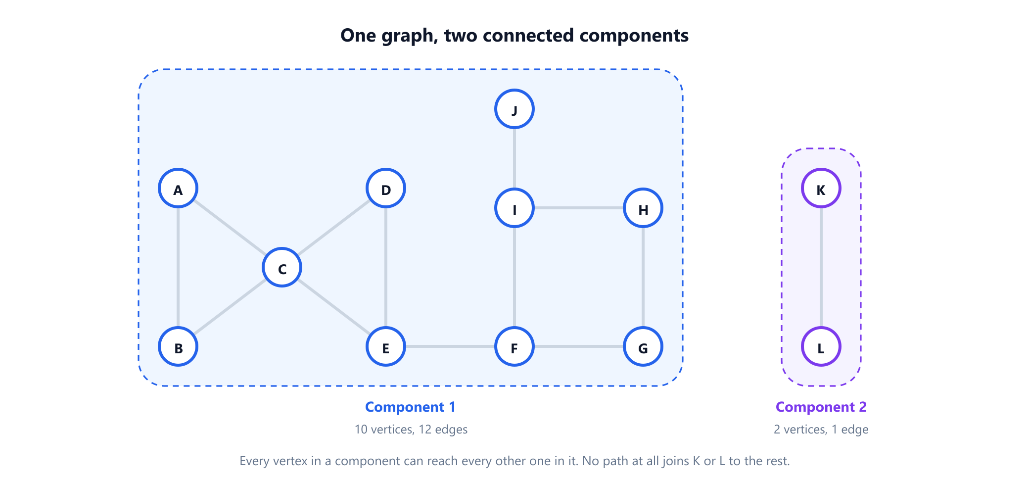
The vocabulary comes from the guide to vertices and edges, and everything here is about undirected graphs until section 11, where direction changes the story.
2. Finding the components
Because components are reachability classes, any graph search finds them. Start a breadth-first or depth-first search at some vertex; everything it reaches is that vertex's component. Then start again from any vertex not yet reached, and repeat until none is left. Each new start is one more component.
from collections import deque

def connected_components(graph):
    """Label every vertex of an undirected graph with the index of its component."""
    label, components = {}, []
    for start in graph:                      # isolated vertices form their own component
        if start in label:
            continue
        label[start] = len(components)
        members, queue = [start], deque([start])
        while queue:
            u = queue.popleft()
            for v in graph[u]:
                if v not in label:
                    label[v] = len(components)
                    members.append(v)
                    queue.append(v)
        components.append(sorted(members))
    return components, label

edges = ['AB', 'BC', 'CA', 'CD', 'DE', 'EC', 'EF', 'FG', 'GH', 'HI', 'IF', 'IJ', 'KL']
graph = {v: [] for v in 'ABCDEFGHIJKL'}
for u, v in edges:
    graph[u].append(v)
    graph[v].append(u)

components, label = connected_components(graph)
print(len(components), components)
# 2 [['A', 'B', 'C', 'D', 'E', 'F', 'G', 'H', 'I', 'J'], ['K', 'L']]
print(label['H'] == label['A'], label['K'] == label['A'])
# True False
Every vertex is labelled once and every edge is looked at twice, once from each end, so the whole job takes O(V + E) time. The outer loop over all vertices is the important line. A single search answers "what can I reach from here", not "how many pieces are there", and forgetting the loop is a common way to get a component count of 1 for a graph that has several.
Two alternatives are worth knowing. If edges arrive one at a time and you only ever add them, a union-find structure keeps the components current in near-constant amortised time per edge: each edge merges the classes of its two ends, and two vertices are in the same component exactly when they have the same root. The idea goes back to Galler and Fischer's 1964 equivalence algorithm. And in image processing, where the "graph" is a grid of pixels, the same problem is called connected-component labelling. Rosenfeld and Pfaltz described a sequential scan for it in 1966. Whether diagonal neighbours count, called 8-connectivity, or only the four straight neighbours do, called 4-connectivity, changes which shapes are one region and which are two.
There is even an algebraic answer. The Laplacian matrix of a graph, degrees on the diagonal and −1 for each edge, has eigenvalue 0 with multiplicity exactly equal to the number of components. For the running example that multiplicity is 2. The connection between eigenvalues and structure is developed in spectral graph theory.
3. What the number of components tells you
Write n for the number of vertices, m for the number of edges and k for the number of components. A handful of facts connect the three, and they are useful as sanity checks on any program that counts components.
A graph withnvertices andkcomponents has at leastn − kedges, with equality exactly when it is a forest.
The proof is a counting argument. Start from n isolated vertices, which is n components, and add the edges one by one. Each edge either joins two different components, lowering the count by one, or lands inside a component and changes nothing. To get down to k components you need at least n − k edges of the first kind, and you have exactly that many when no edge was wasted on closing a cycle. A forest is precisely a graph with no cycles, and a tree is a connected forest, which is why a tree on n vertices has n − 1 edges, as the guide to trees in graph theory proves in several other ways. The running example has 13 ≥ 12 − 2 = 10, with three edges to spare, one for each of its three cycles.
The other direction has a ceiling too. A simple graph with k components has at most C(n − k + 1, 2) edges, reached by putting n − k + 1 vertices in one complete graph and leaving the other k − 1 isolated. A corollary is a quick connectivity test: a simple graph with more than C(n − 1, 2) edges cannot have two components, so it must be connected.
One more fact is a classic exercise with a two-line proof: a graph or its complement is always connected. If G is disconnected, take any two vertices. If they lie in different components of G, they are adjacent in the complement. If they lie in the same component, pick any vertex from another component; it is adjacent to both of them in the complement. Either way they are joined by a path of length at most two. These three facts were checked by brute force over every simple graph on up to six vertices.
4. Bridges: the edges you cannot lose
Connectivity is not only about whether a graph holds together, but about how firmly. A bridge, also called a cut edge, is an edge whose removal increases the number of components. Deleting it splits its component into exactly two pieces, never more, because removing one edge can separate only its two endpoints from each other.
An edge is a bridge if and only if it lies on no cycle.
If an edge uv lies on a cycle, the rest of the cycle is a second route from u to v, so removing the edge disconnects nothing. Conversely, if removing uv leaves u and v connected, the remaining path from v back to u together with uv forms a cycle. So bridges are exactly the edges with no alternative route. Two consequences follow immediately: in a tree every edge is a bridge, and an edge between two vertices joined by a second, parallel edge is never a bridge.
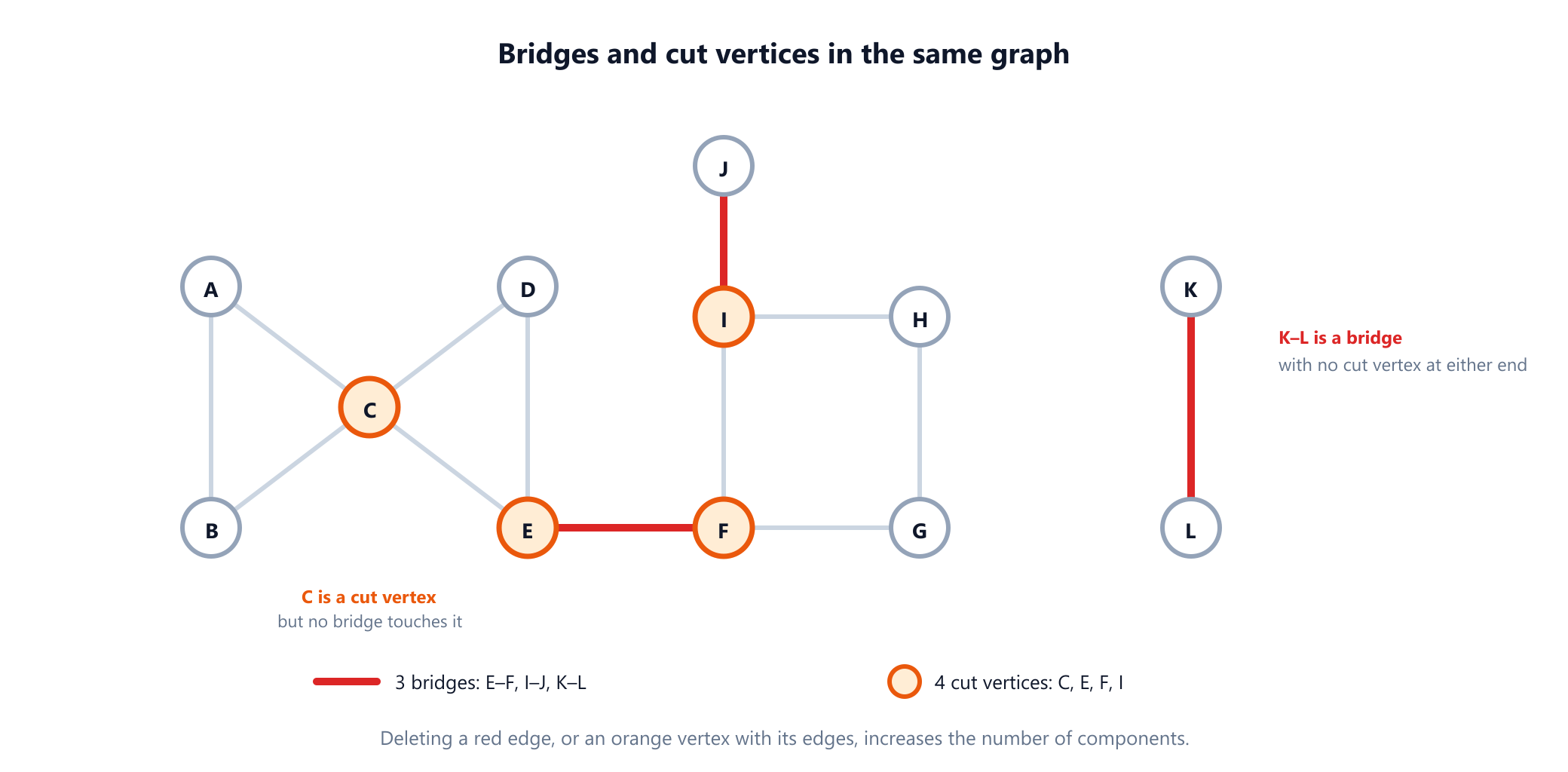
The running example has three bridges: E–F, I–J and K–L. Removing any one of them raises the component count from 2 to 3. Every other edge lies on one of the three cycles, the two triangles and the square.
5. Articulation points: the vertices you cannot lose
An articulation point, also called a cut vertex, is a vertex whose removal, together with its edges, increases the number of components. Equivalently, v is a cut vertex when there are two other vertices u and w in its component such that every path from u to w passes through v.
Unlike a bridge, a cut vertex can split its component into many pieces at once. Remove the centre of a star with five leaves and five components remain. In the running example, removing C leaves three components: {A, B}, everything from D to J, and {K, L}, which was already separate.
Bridges and cut vertices are related, and the relation is a trap worth stating carefully:
- An endpoint of a bridge is a cut vertex unless it has degree 1. Remove
Eand the bridge goes with it, separatingF's side fromD's side. That is whyE,FandIare cut vertices. - A bridge need not have a cut vertex at either end.
K–Lis a bridge, but both ends have degree 1, and removing a leaf never disconnects anything. - A cut vertex need not touch any bridge.
Cjoins two triangles, a shape often called a bowtie. Every edge atClies on a triangle, so none of them is a bridge, yet removingCcutsAandBoff from the rest.
So the running example has four cut vertices, C, E, F and I, and the two ideas are genuinely different: vertex failures and link failures expose different weak points in the same network.
6. One depth-first search finds both
The obvious algorithm deletes each edge, or each vertex, in turn and recounts the components. That costs a full search per candidate, O(E(V + E)) for bridges. In 1972 and 1973 Tarjan, and Hopcroft and Tarjan, showed that a single depth-first search is enough, in O(V + E) total. The method rests on two numbers per vertex.
disc[v]is the time at which the search first reachesv: 0 for the first vertex, 1 for the next, and so on.low[v]is the smallest discovery time that can be reached from the subtree ofvby going down tree edges and then taking at most one back edge.
In an undirected depth-first search every non-tree edge is a back edge: it joins a vertex to one of its ancestors. A back edge is an escape route, a way out of a subtree that does not use the tree edge above it. Both tests ask whether such a route exists. For a tree edge from parent u to child v:
bridge          u–v is a bridge        if  low[v] > disc[u]    nothing below v reaches u or higher
cut vertex      u is a cut vertex     if  low[v] ≥ disc[u]    nothing below v reaches above u
root            the root is a cut vertex  if it has 2 or more children in the DFS tree
The root needs its own rule because nothing lies above it: it separates the graph exactly when the search had to leave it twice, which means its subtrees have no edge between them. Here is the whole method, written iteratively so that a long path cannot overflow Python's call stack:
def bridges_and_cut_vertices(vertices, edges):
    """Tarjan's low-link method, iterative. Edges are (u, v) pairs; parallel edges are allowed."""
    adj = {v: [] for v in vertices}
    for i, (u, v) in enumerate(edges):       # remember edge ids, not just neighbours
        adj[u].append((v, i))
        adj[v].append((u, i))
    disc, low, bridges, cuts, clock = {}, {}, [], set(), 0
    for root in vertices:
        if root in disc:
            continue
        disc[root] = low[root] = clock; clock += 1
        children = 0
        stack = [(root, -1, iter(adj[root]))]  # (vertex, id of the edge we came in by, neighbours)
        while stack:
            u, in_edge, it = stack[-1]
            for v, i in it:
                if i == in_edge:             # skip that one edge, not every edge back to the parent
                    continue
                if v in disc:                # back edge: an escape route up the tree
                    low[u] = min(low[u], disc[v])
                else:                        # tree edge: descend
                    disc[v] = low[v] = clock; clock += 1
                    stack.append((v, i, iter(adj[v])))
                    break
            else:                            # u is finished: report to its parent p
                stack.pop()
                if stack:
                    p = stack[-1][0]
                    low[p] = min(low[p], low[u])
                    if low[u] > disc[p]:
                        bridges.append(edges[in_edge])
                    if low[u] >= disc[p] and p != root:
                        cuts.add(p)
                    if p == root:
                        children += 1
        if children >= 2:                    # the root is a cut vertex only with 2+ DFS children
            cuts.add(root)
    return bridges, sorted(cuts), disc, low

edges = ['AB', 'BC', 'CA', 'CD', 'DE', 'EC', 'EF', 'FG', 'GH', 'HI', 'IF', 'IJ', 'KL']
bridges, cuts, disc, low = bridges_and_cut_vertices('ABCDEFGHIJKL', edges)
print(bridges)
# ['IJ', 'EF', 'KL']
print(cuts)
# ['C', 'E', 'F', 'I']

print(bridges_and_cut_vertices('xy', ['xy', 'xy'])[0])   # a doubled edge is not a bridge
# []
On the running example the search from A happens to walk straight down a path, A, B, C, …, J, and the three non-tree edges C–A, E–C and I–F become back edges. The figure shows the resulting numbers.
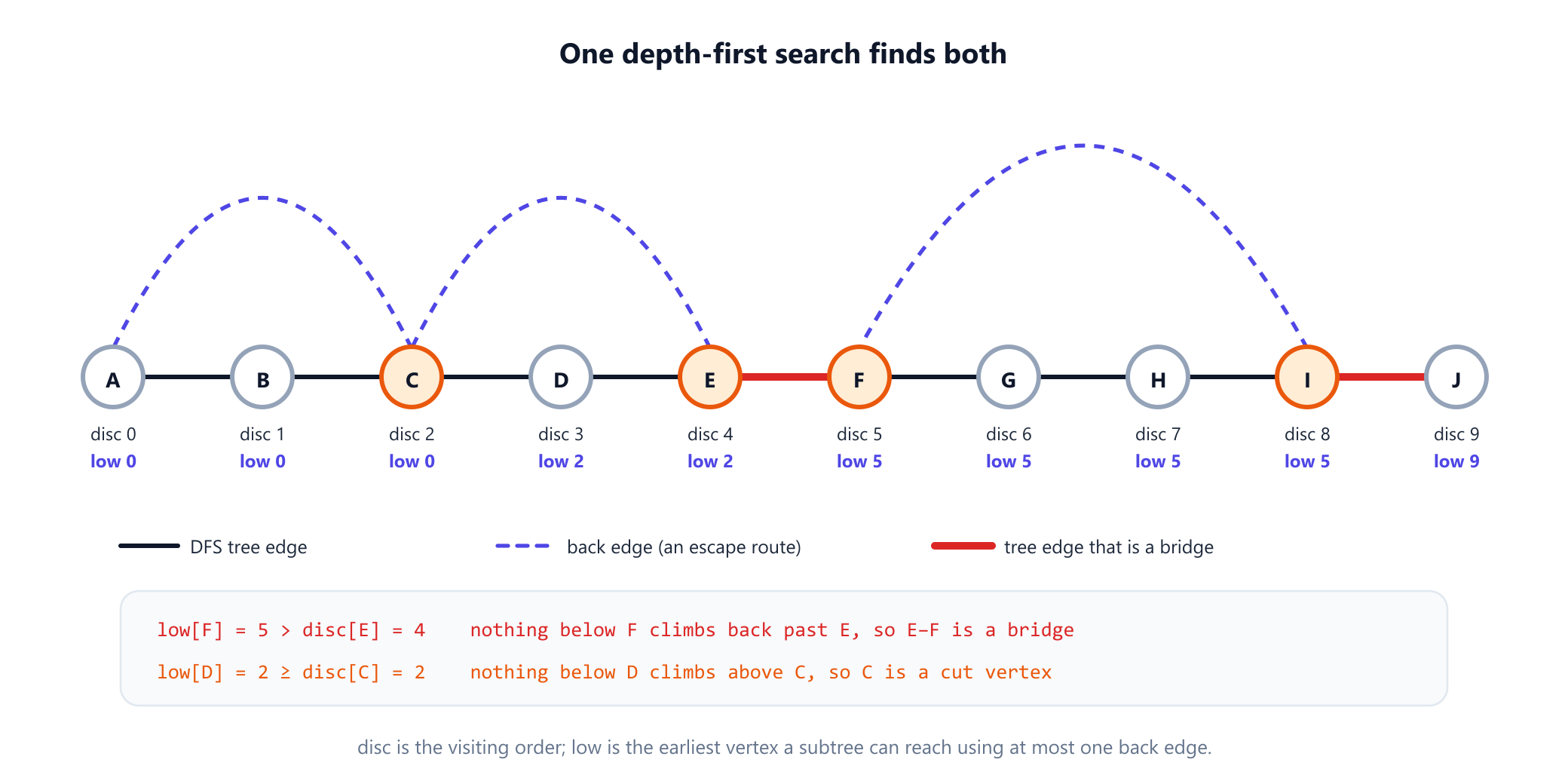
Reading the table against the rules gives every answer. low[F] = 5 is greater than disc[E] = 4, so nothing below F climbs back to E, and E–F is a bridge; I–J is a bridge for the same reason with 9 > 8. low[D] = 2 equals disc[C] = 2: the subtree below C can climb back to C itself but no higher, so C is a cut vertex even though no bridge touches it. And A, the root, has a single child, so it is not.
Watch the low-link values settle
Build the two triangles that share C, run the articulation-point search, and see why C is reported although every edge around it lies on a cycle.
Open the articulation point finder7. Two bugs that pass the simple tests
Low-link code is short, and two of its classic mistakes produce correct answers on most small examples. Both were checked against brute force: the version above agrees with "delete it and recount" on 5,000 random multigraphs.
Skipping the parent vertex instead of the parent edge. When the search looks at the neighbours of v, it must not treat the tree edge it arrived by as a back edge, or every vertex could escape through its own parent. Many implementations skip "the neighbour equal to my parent". That is fine in a simple graph, but with two parallel edges between x and y it skips both of them, and the doubled edge is reported as a bridge although deleting one copy disconnects nothing. Skipping the one edge by its identity, as the code does with in_edge, is correct for multigraphs too.
Using low[w] instead of disc[w] on a back edge. The update along a back edge to w should read disc[w]. Writing low[w] lets the escape route continue past w through edges that belong to a different block. For bridges this happens to be harmless: on 20,000 random graphs the variant never got a bridge wrong. For cut vertices it is not: the same test caught it on 35 of the graphs, and the smallest failure that search found is the pair of triangles sharing C. With low[w], the back edge E–C imports low[C] = 0, so low[D] becomes 0, the test at C fails, and the cut vertex disappears from the output.
8. Blocks and the block-cut tree
Cut vertices split a connected graph into natural pieces. A block is a maximal connected subgraph with no cut vertex of its own: either a 2-connected piece, which stays connected after deleting any one vertex, or a single bridge, or an isolated vertex. Every edge belongs to exactly one block, and two blocks share at most one vertex, which is then a cut vertex. Blocks are also called biconnected components, and Hopcroft and Tarjan's 1973 algorithm finds them in the same single search, by keeping a stack of edges and popping one block each time the cut-vertex test fires.
The running example has six blocks: the triangles {A, B, C} and {C, D, E}, the square {F, G, H, I}, and the three bridges {E, F}, {I, J} and {K, L}.
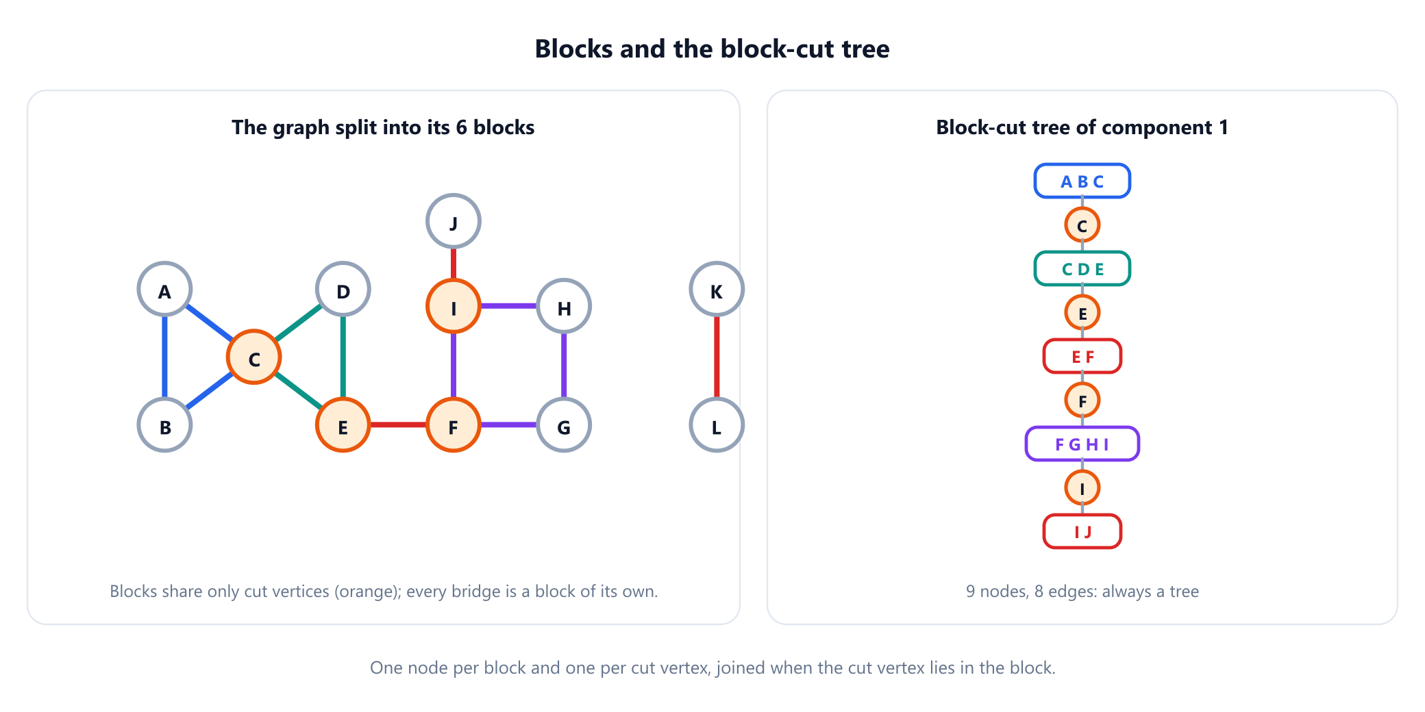
The block-cut tree, introduced by Harary and Prins in 1966, has one node for each block and one for each cut vertex, with an edge whenever the cut vertex lies in the block. For a connected graph it is always a tree. For component 1 it has 5 block nodes and 4 cut-vertex nodes, 9 nodes joined by 8 edges. The tree is the coarse skeleton of the graph: it answers "which failures separate which parts" without looking inside any block.
Bridges give a parallel decomposition. Delete every bridge, and what remains falls into 2-edge-connected components, pieces that survive the loss of any single edge. The example has five: {A, B, C, D, E}, {F, G, H, I}, and the lone vertices {J}, {K} and {L}. Note that the first one is a single 2-edge-connected component but two blocks. The bowtie survives any single edge failure but not the failure of C.
Two classical theorems explain what "no cut vertex" really buys. Whitney showed in 1932 that a graph with at least three vertices is 2-connected exactly when every two vertices are joined by two paths that share no inner vertex, which is the same as saying every two vertices lie on a common cycle. And Robbins proved in 1939 that the edges of a connected graph can be given directions so that every vertex reaches every other exactly when the graph has no bridge, the theorem at the centre of the guide to directed and undirected graphs.
9. Measuring how connected a graph is
Bridges and cut vertices are the first rung of a ladder. The vertex connectivity κ(G) is the smallest number of vertices whose removal disconnects the graph, or leaves a single vertex. The edge connectivity λ(G) is the smallest number of edges whose removal disconnects it. A connected graph with at least three vertices has a cut vertex exactly when κ = 1, and a connected graph with at least two vertices has a bridge exactly when λ = 1. Whitney's inequality of 1932 ties both to the minimum degree δ(G):
κ(G)  ≤  λ(G)  ≤  δ(G)

two triangles sharing C      κ = 1   λ = 2   δ = 2      a cut vertex, but no bridge
component 1 of the example   κ = 1   λ = 1   δ = 1      J hangs on a single edge
any cycle                    κ = 2   λ = 2   δ = 2
The right-hand inequality is easy: deleting the edges at a vertex of minimum degree isolates it. The left-hand one says vertex failures are always at least as dangerous as edge failures, and the bowtie shows the gap can be real.
Menger's theorem of 1927 turns these minimums into maximums. The fewest edges whose removal separates two vertices u and v equals the largest number of paths from u to v that share no edge. The vertex version is the same statement with internally disjoint paths, and it needs u and v to be non-adjacent, since no set of other vertices separates two neighbours. Menger's theorem is a special case of max flow equals min cut, which is also how connectivity is computed in practice.
10. Where this matters
Components, bridges and cut vertices are the vocabulary of failure analysis. Whenever a system can be modelled as things and links, these concepts name its weak points.
| Field | Components mean | A bridge or cut vertex means |
|---|---|---|
| Computer networks | Groups of machines that can talk to each other | A single link or router whose failure partitions the network |
| Roads and rail | Regions reachable from each other | A single bridge, tunnel or junction with no detour |
| Power grids | Islands that can share load | A line or substation that splits the grid if it trips |
| Social networks | Communities with no ties between them | A person who is the only link between two groups |
| Images | Separate objects in a picture | A thin neck where one pixel holds a shape together |
Components also explain one of the most famous results about random graphs. Erdős and Rényi showed in 1960 that if you add random edges to n isolated vertices, the components stay small until the average degree passes 1, and then, quite suddenly, a single giant component containing a constant fraction of all vertices appears. That phase transition, covered in the history of graph theory, is why large real networks almost always have one dominant component with a scattering of small ones around it.
When the graph keeps changing, connectivity becomes a data-structure problem. Insertions alone are easy with union-find. Deletions are much harder, because removing an edge may or may not split a component and finding out seems to need a search. Holm, de Lichtenberg and Thorup showed in 2001 that connectivity, 2-edge-connectivity and biconnectivity can all be maintained under both insertions and deletions in polylogarithmic amortised time per update.
11. Directed graphs: weak and strong connectivity
In a directed graph, "u can reach v" is no longer symmetric, so it is not an equivalence relation, and "the component of v" needs a choice. There are two standard ones.
- Weakly connected components ignore direction: they are the components of the underlying undirected graph, and everything in this article applies to them unchanged.
- Strongly connected components require reachability both ways. "
ureachesvandvreachesu" is an equivalence relation again, and its classes are the strong components, found in linear time by Tarjan's or Kosaraju's algorithm as the guide to strongly connected components explains.
Running the undirected component code on a directed adjacency list gives neither answer. It follows edges only forwards, so the "components" it reports depend on where each search happened to start. Either symmetrise the lists first to get weak components, or use a strong-component algorithm.
12. Common mistakes
| Mistake | Why it is wrong | Fix |
|---|---|---|
| Running one search and calling the graph connected | One search only finds the component of its start vertex | Loop over all vertices and count how many searches you start |
| Forgetting isolated vertices | A vertex with no edges is a component of its own, and edge-list input may not mention it | Build the vertex set separately from the edges |
| "A cut vertex always sits on a bridge" | C in the bowtie is a cut vertex and every edge at it lies on a triangle | Test vertices and edges separately |
| Skipping the parent vertex in low-link code | A doubled edge is then reported as a bridge | Skip the incoming edge by its identity |
Using low[w] on a back edge | Harmless for bridges, but it misses cut vertices such as C | Use disc[w] for back edges and low[v] only for tree children |
| Applying the non-root rule to the root | The root always satisfies low[v] ≥ disc[root] | Make the root a cut vertex only with two or more DFS children |
| Recursing on a long path in Python | The default recursion limit of 1,000 is hit long before memory runs out | Use an explicit stack, as in the code above |
| Using undirected code on a digraph | The result depends on the order of the searches | Decide between weak and strong components first |
13. Glossary
| Term | Meaning |
|---|---|
| Connected graph | A graph with a path between every pair of vertices |
| Connected component | A maximal connected subgraph; a class of the reachability relation |
| Bridge, cut edge | An edge whose removal increases the number of components; an edge on no cycle |
| Articulation point, cut vertex | A vertex whose removal increases the number of components |
| Back edge | A non-tree edge of a depth-first search, joining a vertex to an ancestor |
| Low-link value | The smallest discovery time reachable from a subtree using at most one back edge |
| Block, biconnected component | A maximal connected subgraph with no cut vertex of its own |
| Block-cut tree | The tree with a node per block and per cut vertex |
| 2-edge-connected component | A piece left after deleting every bridge |
Vertex connectivity κ | The fewest vertices whose removal disconnects the graph |
Edge connectivity λ | The fewest edges whose removal disconnects the graph |
| Giant component | A component containing a constant fraction of all vertices |
14. Frequently asked questions
What is a connected component of a graph?
A connected component is a maximal set of vertices in which every vertex can reach every other by a path, together with the edges between them. Components are the classes of the reachability relation, so every vertex belongs to exactly one, and an isolated vertex is a component on its own. A graph is connected exactly when it has one component.
How do you find the connected components of a graph?
Start a breadth-first or depth-first search at any vertex; everything it reaches is one component. Then start a new search from any vertex not yet reached, and repeat until every vertex is labelled. The number of searches started is the number of components, and the whole procedure takes O(V + E) time. If edges only ever get added, a union-find structure keeps the components up to date instead.
What is a bridge in a graph?
A bridge, or cut edge, is an edge whose removal increases the number of connected components. An edge is a bridge exactly when it lies on no cycle, so every edge of a tree is a bridge and an edge with a parallel copy never is. Deleting a bridge splits its component into exactly two pieces.
What is an articulation point?
An articulation point, or cut vertex, is a vertex whose removal, together with its edges, increases the number of connected components. Unlike a bridge it can split a component into many pieces: removing the centre of a star with five leaves leaves five components. A cut vertex need not touch any bridge, as two triangles sharing one vertex show.
How does Tarjan’s algorithm find bridges and articulation points?
It runs one depth-first search and records two numbers per vertex: disc, the order in which the vertex was first reached, and low, the smallest disc reachable from its subtree using at most one back edge. A tree edge from u to a child v is a bridge when low[v] > disc[u]. A non-root u is a cut vertex when some child v has low[v] ≥ disc[u], and the root is a cut vertex when it has two or more children in the search tree. Everything runs in O(V + E) time.
What is the difference between a bridge and an articulation point?
A bridge is an edge and an articulation point is a vertex; each is a single point of failure of a different kind. They often come together, since an endpoint of a bridge is a cut vertex unless it has degree 1, but neither implies the other. A lone edge between two leaves is a bridge with no cut vertex, and the shared vertex of two triangles is a cut vertex with no bridge.
15. References
The definitions, theorems and attributions above come from these sources, listed in chronological order.
- Menger, K. (1927). "Zur allgemeinen Kurventheorie." Fundamenta Mathematicae 10, 96 to 115. Disjoint paths and separating sets.
- Whitney, H. (1932). "Congruent Graphs and the Connectivity of Graphs." American Journal of Mathematics 54(1), 150 to 168.
- Whitney, H. (1932). "Non-separable and Planar Graphs." Transactions of the American Mathematical Society 34(2), 339 to 362. With the paper above, the inequality between vertex connectivity, edge connectivity and minimum degree, and the characterisation of 2-connected graphs by disjoint paths.
- Robbins, H. E. (1939). "A Theorem on Graphs, with an Application to a Problem of Traffic Control." American Mathematical Monthly 46(5), 281 to 283.
- Erdős, P. and Rényi, A. (1960). "On the Evolution of Random Graphs." Publications of the Mathematical Institute of the Hungarian Academy of Sciences 5, 17 to 61. The giant component.
- Galler, B. A. and Fischer, M. J. (1964). "An Improved Equivalence Algorithm." Communications of the ACM 7(5), 301 to 303. The union-find idea for merging classes.
- Harary, F. and Prins, G. (1966). "The Block-Cutpoint-Tree of a Graph." Publicationes Mathematicae Debrecen 13, 103 to 107.
- Rosenfeld, A. and Pfaltz, J. L. (1966). "Sequential Operations in Digital Picture Processing." Journal of the ACM 13(4), 471 to 494. Connected-component labelling of images.
- Tarjan, R. E. (1972). "Depth-First Search and Linear Graph Algorithms." SIAM Journal on Computing 1(2), 146 to 160.
- Hopcroft, J. E. and Tarjan, R. E. (1973). "Algorithm 447: Efficient Algorithms for Graph Manipulation." Communications of the ACM 16(6), 372 to 378. Biconnected components and cut vertices in linear time.
- Tarjan, R. E. (1974). "A Note on Finding the Bridges of a Graph." Information Processing Letters 2(6), 160 to 161.
- Holm, J., de Lichtenberg, K. and Thorup, M. (2001). "Poly-logarithmic Deterministic Fully-Dynamic Algorithms for Connectivity, Minimum Spanning Tree, 2-Edge, and Biconnectivity." Journal of the ACM 48(4), 723 to 760.
- Diestel, R. (2017). Graph Theory, 5th edition. Graduate Texts in Mathematics 173. Berlin: Springer.
Find the weak links yourself
Draw a network, run the bridge finder, and watch the depth-first search mark every edge that has no detour. Then add one edge and see a bridge disappear.
Open the visualizer