
Table of Contents
- 1. A tree has seven definitions, and they are all the same one
- 2. The equivalence theorem, and how its proof works
- 3. The leaf lemma
- 4. Forests, and counting components for free
- 5. Spanning trees
- 6. Counting labelled trees: Cayley's formula
- 7. The Prüfer bijection, worked end to end
- 8. The matrix-tree theorem
- 9. Unlabelled trees: a much harder question
- 10. Centres, radius and diameter
- 11. Distance in trees, and the double BFS trick
- 12. Free trees, rooted trees, ordered trees
- 13. Where trees show up in computing
- 14. Common mistakes
- 15. Glossary
- 16. Frequently asked questions
- 17. References
1. A tree has seven definitions, and they are all the same one
Ask three people to define a tree and you will get three answers. One says it is a connected graph with no cycles. Another says it is a graph with exactly one path between any two vertices. A third says it is a connected graph with n - 1 edges. All three are right, and so are four more definitions besides, because these conditions are equivalent: any graph satisfying one satisfies all of them.
That is unusual, and it is the reason trees are the most useful special case in the subject. A structure with seven equivalent characterisations gives you seven different ways to prove something about it, and in practice you pick whichever one makes the proof shortest.
Start with the standard definition, the one in Diestel and in Bondy and Murty:
A tree is a connected acyclic graph. A graph whose components are all trees is a forest. A vertex of degree 1 in a tree is a leaf.
Everything below is about a finite simple, undirected graph, which is the standard setting. A tree cannot have a loop or a parallel edge anyway, since either one is a cycle.
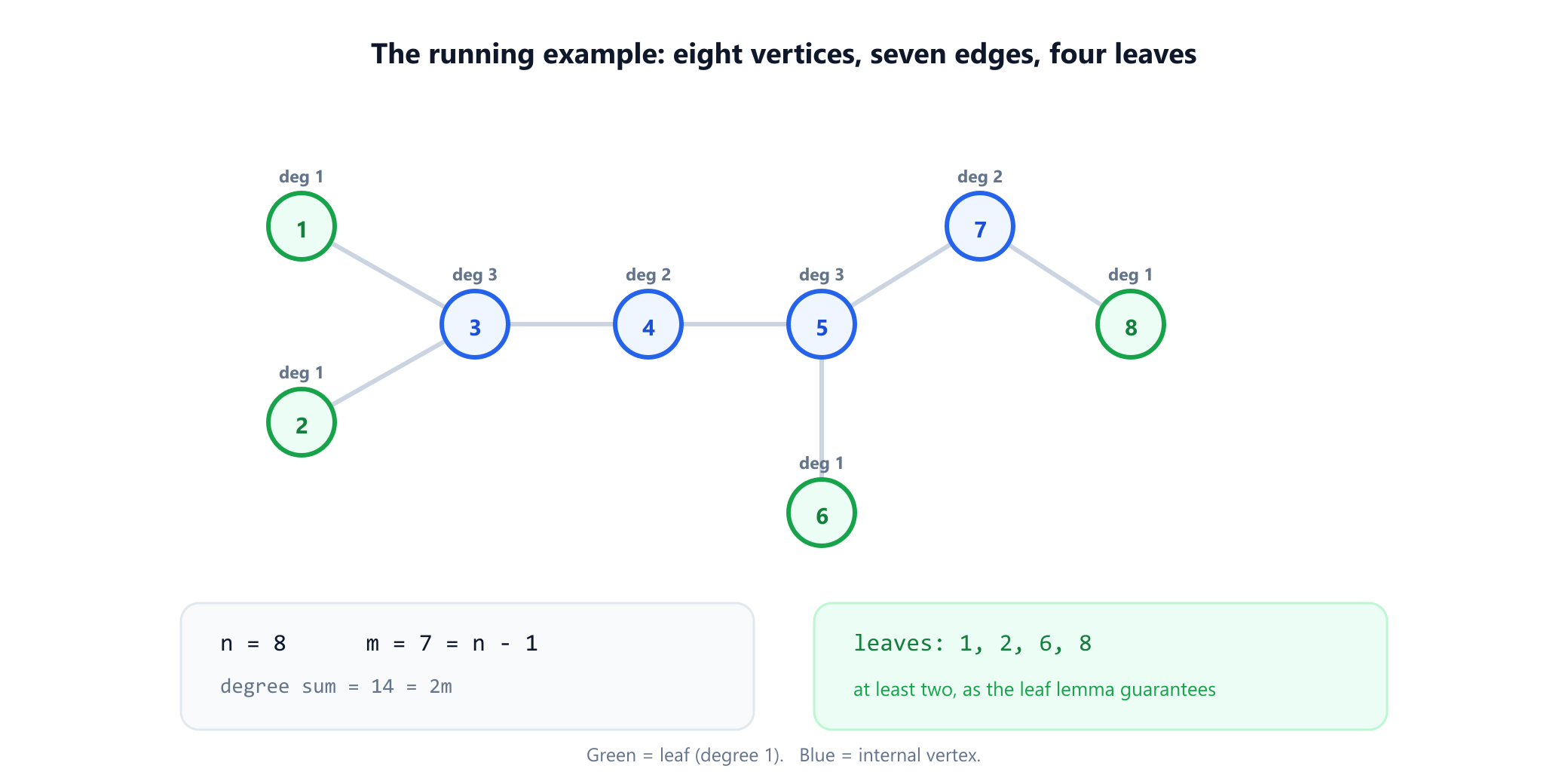
Written out, the running example is
V = {1, 2, 3, 4, 5, 6, 7, 8}
E = { {1,3}, {2,3}, {3,4}, {4,5}, {5,6}, {5,7}, {7,8} }

degrees   1:1   2:1   3:3   4:2   5:3   6:1   7:2   8:1
n = 8     m = 7 = n - 1      degree sum = 14 = 2m      leaves: 1, 2, 6, 8
2. The equivalence theorem, and how its proof works
Here is the result in full. It appears in essentially this form in West, in Bondy and Murty, and in Diestel, and it is worth memorising because each line is a tool.
Theorem. For a graphGonnvertices, the following are equivalent:
(1)Gis a tree, that is, connected and acyclic.
(2) Any two vertices ofGare joined by exactly one path.
(3)Gis connected and hasn - 1edges.
(4)Gis acyclic and hasn - 1edges.
(5)Gis connected, and removing any single edge disconnects it (minimally connected).
(6)Gis acyclic, and adding any single edge creates a cycle (maximally acyclic).
(7)Gis connected and every edge is a bridge.
The proof is not one argument but a cycle of implications, each of them short. It is worth seeing the shape, because it explains why the conditions feel so different from one another and yet describe the same object.
| Step | Why it holds |
|---|---|
| (1) → (2) | Connectivity gives at least one path. If two distinct paths joined the same pair, their union would contain a cycle, contradicting acyclicity. |
| (2) → (5) | One path between every pair means connected. Deleting the edge {u, v} destroys the only path from u to v, so the graph falls apart. |
| (5) → (1) | If a cycle existed, any edge of it could be deleted while leaving the graph connected, since the rest of the cycle still joins its ends. So there is no cycle. |
| (1) → (3) | Induction on n. A tree has a leaf (section 3); delete it and you have a tree on n - 1 vertices, which by induction has n - 2 edges. Put the leaf back and you have n - 1. |
| (3) → (4) | Suppose G were connected with n - 1 edges and still had a cycle. Delete one edge of that cycle: the graph stays connected, but now has only n - 2 edges, and a connected graph on n vertices needs at least n - 1. The contradiction rules out the cycle. |
| (4) → (1) | An acyclic graph with k components and n vertices has exactly n - k edges (section 4). With n - 1 edges, k = 1, so it is connected. |
| (1) ↔ (6) | Adding {u, v} to a tree closes the unique existing u to v path into a cycle. Conversely, maximal acyclicity forces connectivity, since two vertices in different components could be joined without creating any cycle. |
Two of these deserve emphasis because they are the ones people actually use.
"Connected and n - 1 edges" is the cheapest test. Counting edges is O(m) and a connectivity check is O(n + m), so you can decide treehood in linear time without ever looking for a cycle. Note that neither half suffices alone: a triangle plus an isolated vertex has 4 vertices and 3 edges but is not a tree, and neither is a 4-cycle, which is connected with 4 edges.
"Minimally connected" and "maximally acyclic" are the same object seen from two directions. A tree sits exactly on the boundary: it has as few edges as connectivity allows and as many as acyclicity allows. That is why trees turn up whenever a problem asks for a cheapest connecting structure, which is precisely the minimum spanning tree problem.
All seven conditions hold on the running example, and each was checked directly: it is connected, acyclic, has 7 edges on 8 vertices, has exactly one path between each of the 28 vertex pairs, every one of its 7 edges is a bridge, and every one of the 21 missing edges closes a cycle when added.
3. The leaf lemma
One small result carries most of the inductive proofs in the subject.
Leaf lemma. Every finite tree with at least two vertices has at least two leaves.
The proof is a favourite because it uses nothing but the definition. Take a longest path P in the tree, say from u to v. Such a path exists because the tree is finite. Now consider u. If u had a neighbour w outside P, then P could be extended by that edge, contradicting maximality. If u had a second neighbour on P, that would close a cycle, contradicting acyclicity. So u has exactly one neighbour and is a leaf, and the same argument applies to v.
Two consequences follow immediately and both are used constantly:
- Induction on trees always has a base case to remove. Delete a leaf from a tree and what remains is a tree with one fewer vertex. That single move is the engine of the proof that a tree has
n - 1edges, of the Prüfer encoding in section 7, and of the centre-finding algorithm in section 10. - The bound is tight. A path has exactly two leaves, so "at least two" cannot be improved in general. At the other extreme, the star
K1,n-1hasn - 1leaves.
The running example has four leaves, 1, 2, 6 and 8, comfortably more than the guaranteed two. A useful sanity check when debugging tree code: if your structure claims to be a tree and reports fewer than two leaves, something is wrong, and the usual culprit is an accidental cycle.
The lemma is also exactly what fails on infinite graphs. The one-way infinite path has a single leaf and the two-way infinite path has none at all, which is one of the cleanest illustrations of what finiteness was buying, covered in the guide to finite and infinite graphs.
4. Forests, and counting components for free
A forest is an acyclic graph, connected or not. Every component of a forest is a tree, and that gives a counting identity worth knowing by heart:
A forest withnvertices andkcomponents has exactlyn - kedges.
The proof is one line: each component is a tree, so a component with ni vertices contributes ni - 1 edges, and summing over the k components gives n - k. Setting k = 1 recovers the tree case.
Read the identity backwards and it becomes a tool rather than a fact:
k = n - m        the number of components of a forest,
                 computed from its size alone, with no traversal
That is genuinely useful. If you know a graph is acyclic, counting its vertices and edges tells you how many pieces it is in without running a search. It is also the identity behind the standard union-find invariant: every successful union merges two components and adds one edge, so the running count n - (unions so far) is the number of components at any moment.
One warning. The identity assumes acyclicity. For a general graph, m ≥ n - k always holds, with equality exactly when the graph is a forest, so a graph with more edges than n - k necessarily contains a cycle. That inequality is the fastest way to prove a graph has a cycle without finding one: if m ≥ n, there is a cycle somewhere.
5. Spanning trees
A spanning tree of a connected graph G is a subgraph that is a tree and includes every vertex of G. It is the minimal skeleton that keeps the graph in one piece.
Every connected finite graph has one, and the constructive proof is worth knowing because it is also an algorithm: while a cycle exists, delete any edge of it. Deleting a cycle edge cannot disconnect the graph, since the rest of the cycle still joins its endpoints, and the process terminates because each step removes an edge. What remains is connected and acyclic. Equivalently, and more practically, the tree of discovery edges produced by any BFS or DFS traversal is already a spanning tree, found in O(n + m).
Three facts about spanning trees that come up repeatedly:
- Every spanning tree has exactly
n - 1edges, whatever the graph looked like. So on an unweighted graph all spanning trees tie, and the minimum spanning tree problem is only interesting once edges carry weights. - The number of spanning trees can be enormous. The complete graph
Knhasnn-2of them, which is Cayley's formula again, viewed from the spanning-tree side. - A tree is its own unique spanning tree. Obvious once stated, and a useful degenerate case for testing code: any spanning-tree counter should return exactly 1 on a tree, which the matrix-tree computation in section 8 confirms for the running example.
For infinite graphs the statement "every connected graph has a spanning tree" is still true but needs the axiom of choice, and is in fact equivalent to it. That boundary is discussed in the finite and infinite graphs guide.
6. Counting labelled trees: Cayley's formula
How many different trees can be built on a fixed set of n labelled vertices? The answer is one of the most quotable results in combinatorics, published by Arthur Cayley in 1889.
Cayley's formula. The number of labelled trees onnvertices isnn-2.
The first few values grow fast, and they are worth seeing because the smallest ones can be checked by hand:
| n | nn-2 | Check |
|---|---|---|
| 2 | 1 | The single edge, and nothing else is possible |
| 3 | 3 | A path on 3 vertices, once for each choice of middle vertex |
| 4 | 16 | Verified by exhaustive enumeration of all edge subsets |
| 5 | 125 | Verified the same way |
| 6 | 1296 | Already past hand-checking |
The counts for n = 4 and n = 5 above are not quoted from a book; they were produced by enumerating every subset of n - 1 edges from the C(n, 2) candidates and keeping the connected ones, giving 16 and 125 exactly.
A word on what "labelled" means, because the distinction is the whole subject of section 9. Cayley counts trees whose vertices are distinguishable, so the path 1 - 2 - 3 and the path 2 - 1 - 3 are different trees even though they have the same shape. Strip the labels and there is only one shape of tree on three vertices.
Several proofs of the formula exist, including a double-counting argument on rooted forests and a determinant argument via the matrix-tree theorem. The most illuminating is a bijection, and it is short enough to work through completely.
7. The Prüfer bijection, worked end to end
Heinz Prüfer gave a proof of Cayley's formula in 1918 by constructing an explicit bijection between labelled trees on n vertices and sequences of length n - 2 drawn from {1, …, n}. Since there are exactly nn-2 such sequences, the formula follows at once.
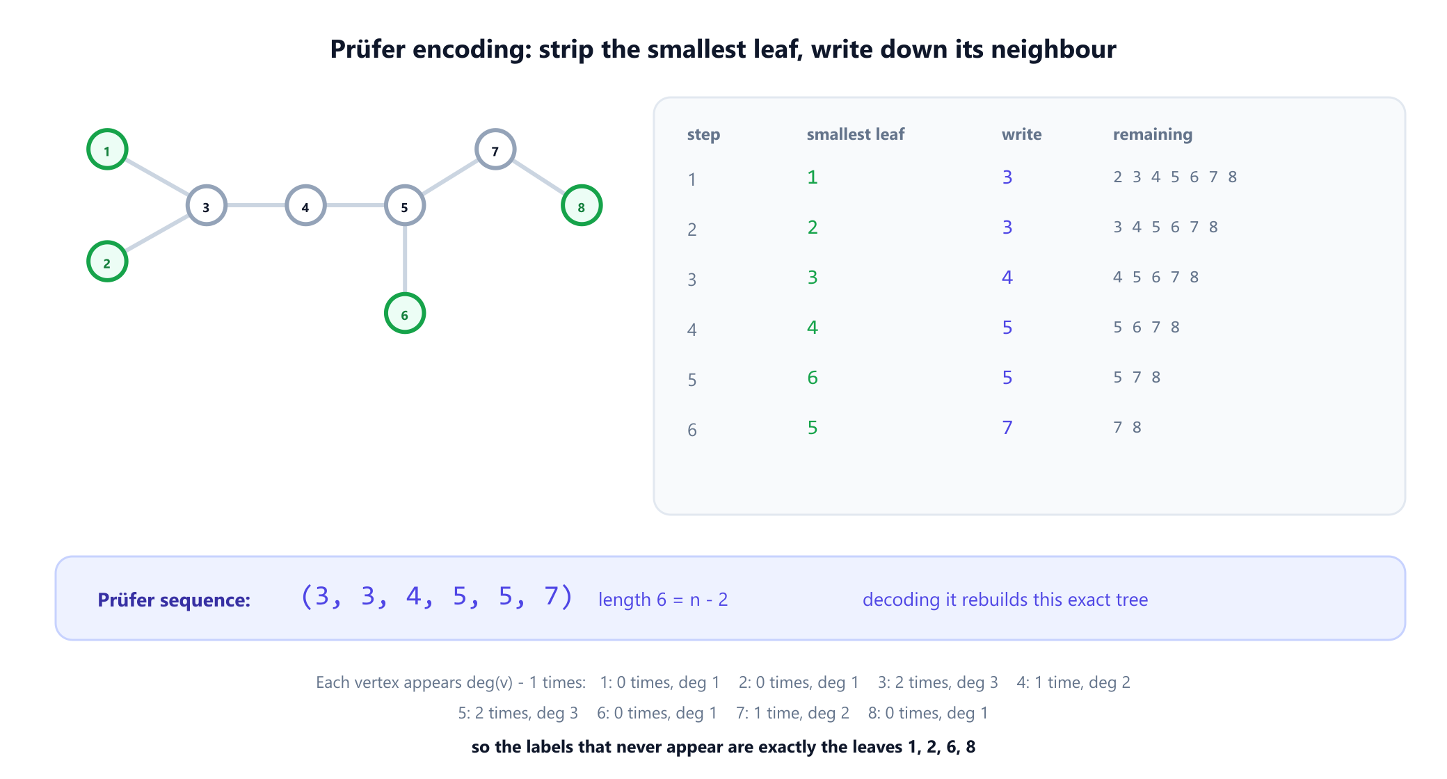
Encoding. While more than two vertices remain, find the leaf with the smallest label, write down the label of its unique neighbour, and delete the leaf. Stop when two vertices are left. On the running example this produces, step by step:
remove leaf 1  →  write 3        remaining: 2,3,4,5,6,7,8
remove leaf 2  →  write 3        remaining: 3,4,5,6,7,8
remove leaf 3  →  write 4        remaining: 4,5,6,7,8
remove leaf 4  →  write 5        remaining: 5,6,7,8
remove leaf 6  →  write 5        remaining: 5,7,8
remove leaf 5  →  write 7        remaining: 7,8

Prüfer sequence:  (3, 3, 4, 5, 5, 7)        length 6 = n - 2
Decoding. The inverse runs the same idea backwards. Give every vertex a counter equal to one plus the number of times it appears in the sequence, which will be its degree. Then repeatedly take the smallest vertex whose counter is 1 and is not yet used, join it to the first remaining entry of the sequence, and decrement both counters. When the sequence is exhausted, join the two vertices still holding a counter of 1. Running this on (3, 3, 4, 5, 5, 7) returns exactly the original edge set, which is what makes the correspondence a bijection rather than merely a summary.
The single most useful property of the encoding is this:
Vertexvappears in the Prüfer sequence exactlydeg(v) - 1times. In particular, the leaves are precisely the labels that never appear.
Check it against the running example. Vertex 3 has degree 3 and appears twice; vertex 5 has degree 3 and appears twice; vertices 4 and 7 have degree 2 and appear once each; and the leaves 1, 2, 6 and 8 appear not at all. That correspondence turns questions about degree sequences into questions about how often symbols occur in a string, which is why Prüfer sequences are the standard tool for counting trees with prescribed degrees and for sampling a labelled tree uniformly at random: generate a random sequence of length n - 2 and decode it.
8. The matrix-tree theorem
Cayley's formula counts spanning trees of the complete graph. Kirchhoff's matrix-tree theorem, which predates it by four decades and came out of his work on electrical networks in 1847, counts the spanning trees of any graph.
Build the Laplacian matrix L = D - A, where D is the diagonal matrix of degrees and A is the adjacency matrix. Then:
Matrix-tree theorem. Delete any one row and the corresponding column fromL. The determinant of the remaining(n-1) × (n-1)matrix is the number of spanning trees of the graph. The choice of which row and column to delete does not matter.
Three computations make the theorem concrete, and all three were carried out rather than quoted:
| Graph | Spanning trees | Cross-check |
|---|---|---|
K4, the complete graph on 4 vertices | 16 | Agrees with Cayley: 44-2 = 16 |
C4, the 4-cycle | 4 | Delete any one of the 4 edges and a spanning tree remains |
| The running example tree | 1 | A tree is its own only spanning tree |
The cycle case is the one to hold on to as intuition: a cycle on k vertices has exactly k spanning trees, one for each edge you choose to drop. The theorem also explains a remark from the guide to multigraphs: parallel edges genuinely change the spanning tree count, because they enter the Laplacian as off-diagonal multiplicities, so two vertices joined by two parallel edges have two spanning trees rather than one.
9. Unlabelled trees: a much harder question
Cayley's formula is clean because labels make trees easy to tell apart. Ask instead how many trees there are up to isomorphism, meaning how many distinct shapes exist, and the problem becomes genuinely hard.
| n | Labelled trees (nn-2) | Unlabelled trees |
|---|---|---|
| 1 | 1 | 1 |
| 2 | 1 | 1 |
| 3 | 3 | 1 |
| 4 | 16 | 2 |
| 5 | 125 | 3 |
| 6 | 1296 | 6 |
| 7 | 16807 | 11 |
The two columns tell completely different stories. The labelled count has a one-line closed form; the unlabelled count has none. There is no known formula for the number of trees on n vertices up to isomorphism, only a generating-function treatment and an asymptotic result due to Richard Otter in 1948, which shows the count grows like C · αn n-5/2 for constants worked out numerically.
The reason for the gap is symmetry. Dividing the labelled count by n! would be right only if every tree had trivial automorphism group, and most do not: a path can be reflected, a star can have its leaves permuted arbitrarily, and each symmetry means several labellings collapse to the same shape. Counting orbits under the symmetric group is exactly the hard part, and it is the reason the problem needs Pólya's enumeration machinery rather than a formula.
For a working programmer the practical form of this distinction is tree isomorphism testing: deciding whether two trees have the same shape. Unlike general graph isomorphism, this is solvable in linear time, by canonically hashing each subtree bottom up from the leaves and comparing the results at the centre. That the general problem is hard while the tree case is easy is one more instance of the pattern running through this whole article.
10. Centres, radius and diameter
The eccentricity of a vertex is its greatest distance to any other vertex. The radius is the smallest eccentricity in the graph, the diameter the largest, and the centre is the set of vertices attaining the radius. For trees these have unusually clean behaviour, first worked out by Camille Jordan in 1869.
Jordan's theorem. The centre of a tree consists of either one vertex or two adjacent vertices.
Never three, never two non-adjacent ones. Compare that with a cycle, where every vertex is in the centre, and the sharpness of the tree case is clear.
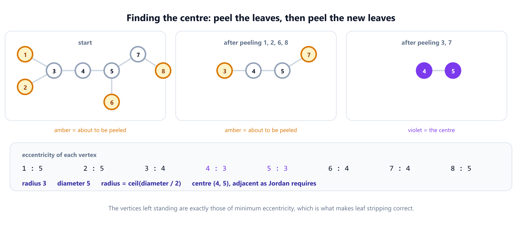
The proof doubles as the algorithm. Repeatedly delete all current leaves simultaneously. Every deletion reduces the eccentricity of every surviving vertex by exactly 1, so it preserves which vertices are minimal, and the process ends with one or two vertices left. On the running example:
start        1 2 3 4 5 6 7 8
strip leaves 1, 2, 6, 8   →   remaining  3 4 5 7
strip leaves 3, 7         →   remaining  4 5      ← the centre

eccentricities   1:5  2:5  3:4  4:3  5:3  6:4  7:4  8:5
radius 3     diameter 5     centre {4, 5}, adjacent as Jordan requires
The leaf-stripping result was checked against a direct computation of all eight eccentricities, and the two agree exactly: the vertices of minimum eccentricity are precisely 4 and 5. The algorithm runs in O(n), which is why it is the standard way to root a tree "in the middle", for instance before canonical hashing in isomorphism testing.
One more identity holds in trees and is worth remembering:
radius = ⌈diameter / 2⌉ here: 3 = ⌈5 / 2⌉It follows because a tree's diameter is realised by a unique path, and the centre sits at that path's midpoint. In a general graph only the weaker radius ≤ diameter ≤ 2 · radius holds.
11. Distance in trees, and the double BFS trick
Because there is exactly one path between any two vertices, distance in a tree is simpler than in any other class of graph. There is nothing to optimise: the unique path is the shortest path, so no weights, no priority queue and no Dijkstra are needed to find it.
That uniqueness gives a neat and widely used algorithm for the diameter:
Double BFS. Run a breadth first search from any vertex and letabe a farthest vertex found. Run a second search fromaand letbbe a farthest vertex from it. Then the path fromatobis a diameter, anddist(a, b)is the diameter's length.
Two linear passes, no weights, no cleverness. On the running example, starting at vertex 1 the search reaches vertex 8 as a farthest vertex, and a second search from 8 returns vertex 1 at distance 5, matching the true diameter computed by taking the maximum over all eccentricities.
The reason it works is worth stating, because the trick fails on general graphs and people transplant it anyway. The key claim is that a farthest vertex from any starting point is always an endpoint of some diameter. In a tree this holds because the unique paths force the farthest vertex to lie at the end of the longest path; in a graph with cycles the claim is simply false, and the two-pass method can return an underestimate. On a general graph, computing the diameter needs all-pairs distances.
Some other distance facts that hold in trees and nowhere else in general:
- Removing any edge splits the tree into exactly two components, since every edge is a bridge. That is what makes divide-and-conquer on trees, such as centroid decomposition, work so cleanly.
- The path between two vertices can be recovered from parent pointers alone once the tree is rooted, in time proportional to the path length, which underpins lowest-common-ancestor techniques.
- Distances satisfy the four-point condition, a metric identity characterising exactly those distance matrices that come from trees, which is the basis of phylogenetic tree reconstruction from genetic distance data.
12. Free trees, rooted trees, ordered trees
Everything so far has been about free trees: connected acyclic graphs with no distinguished vertex and no ordering among the neighbours of any vertex. Computer science almost always works with something more structured, and Knuth's The Art of Computer Programming is careful to separate the three levels, because the counts differ at every one.
| Object | Extra structure | Example count on 3 nodes |
|---|---|---|
| Free tree | None. Just a connected acyclic graph | 1 shape |
| Rooted tree | One vertex is designated the root, which orients every edge away from it | 2 shapes: a path rooted at an end, or at the middle |
| Ordered tree | The children of each node have a left-to-right order | 2 shapes, and the distinction bites from 4 nodes upwards |
Rooting is not a change to the graph, it is a change to the question. The underlying edge set is identical; what a root adds is a direction, and with it the whole vocabulary of parent, child, ancestor, descendant, depth and height, which the companion guide on rooted trees covers in detail along with the standard traversals.
The counting difference is the sharpest way to see that these really are different objects. Ordered binary trees on n nodes are counted by the Catalan numbers, giving 1, 1, 2, 5, 14, 42 for n = 0 to 5, whereas free trees on the same number of vertices are far fewer. Every extra piece of structure you insist on multiplies the number of distinct objects.
A practical note that follows from section 10: when an algorithm needs a root and none is given, rooting at the centre is usually the right default. It minimises the height, which bounds the depth of any recursion you run over the tree.
13. Where trees show up in computing
Trees are the most common structure in computing that is genuinely a graph, and it is worth separating the cases where the tree is the data from those where it is a certificate produced by an algorithm.
Trees as data. The hierarchy is the point:
- File systems. Directories and files form a rooted tree, at least until symbolic links and hard links are allowed, at which point it becomes a general graph and the guarantee of a unique path is lost. That is exactly why link loops break naive directory walkers.
- Parse trees and abstract syntax trees. Every compiler front end produces one. Being a tree is what makes recursive evaluation well founded: a subexpression cannot contain itself.
- The DOM. An HTML document is an ordered rooted tree, and CSS selectors are queries over ancestor and sibling relations in it.
- Search trees, tries and heaps. Binary search trees, B-trees and tries are trees whose shape is constrained to bound the depth, which is exactly the height of the rooted tree.
- Decision trees. Each internal node tests a feature and each leaf carries a prediction; the unique root-to-leaf path is the explanation of the model's output.
Trees as certificates. Here the tree is the output of an algorithm and encodes a proof:
- BFS and DFS trees. Every traversal of a connected graph produces a spanning tree of discovery edges. The BFS tree additionally certifies shortest distances in an unweighted graph, and the DFS tree's back edges are what let you detect cycles and find bridges.
- Shortest path trees. Dijkstra's algorithm outputs one: a spanning tree in which the path from the source to any vertex is a shortest path. Note it is generally not a minimum spanning tree, and confusing the two is a classic error.
- Minimum spanning trees. Kruskal, Prim and Borůvka each certify the cheapest connecting subgraph, discussed in the MST guide.
- Union-find forests. The disjoint-set structure literally is a forest, and path compression is an operation that flattens its trees to keep the height near constant.
- Merkle trees. Hash trees in version control and distributed systems use the unique-path property so that a single leaf change propagates along exactly one path to the root, making verification logarithmic.
One clarification worth making, because the terminology misleads people: a Git commit history is not a tree. A merge commit has two parents, so the history is a directed acyclic graph. Git's "tree" objects are something else entirely, namely the directory snapshots. The distinction between a DAG and a tree is precisely that a tree has a unique path between any two nodes, and a merge destroys that.
14. Common mistakes
- Checking only one half of the definition. "Connected" alone admits cycles; "
n - 1edges" alone admits a triangle plus an isolated vertex. You need a pair of conditions from the theorem in section 2, and connected plusn - 1edges is the cheapest. - Assuming a shortest path tree is a minimum spanning tree. They optimise different things: one minimises each distance from the source, the other minimises total edge weight. They frequently differ.
- Using the double BFS diameter trick on a graph with cycles. It is valid only on trees, where the unique-path property makes a farthest vertex a diameter endpoint. On general graphs it can silently underestimate.
- Confusing labelled and unlabelled counts. There are 125 labelled trees on 5 vertices and only 3 shapes. Dividing by
n!does not convert between them, because trees have symmetries. - Forgetting that rooting changes nothing structurally. A root adds a question, not an edge. The underlying free tree is unchanged, so any structural fact proved for free trees still applies.
- Expecting the leaf lemma on infinite trees. The two-way infinite path is acyclic and connected with no leaf at all.
- Treating a DAG as a tree. A DAG can have several paths between two nodes; a tree cannot. Any algorithm relying on path uniqueness, including naive memoisation keyed on a node, will misbehave.
- Building a "tree" that has a cycle. The fastest runtime check is the edge count: if a supposed tree on
nvertices does not have exactlyn - 1edges, stop and look for the bug.
15. Glossary
| Term | Meaning |
|---|---|
| Tree | A connected acyclic graph; equivalently any of the seven conditions in section 2 |
| Forest | An acyclic graph; every component is a tree. With n vertices and k components it has n - k edges |
| Leaf | A vertex of degree 1. Every finite tree with at least 2 vertices has at least 2 |
| Spanning tree | A subgraph that is a tree and touches every vertex of the host graph |
| Bridge | An edge whose removal disconnects the graph. In a tree, every edge is one |
| Eccentricity | The greatest distance from a vertex to any other |
| Radius, diameter | The minimum and maximum eccentricity. In a tree, radius = ⌈diameter / 2⌉ |
| Centre | The vertices of minimum eccentricity. In a tree this is one vertex or two adjacent ones |
| Cayley's formula | There are nn-2 labelled trees on n vertices |
| Prüfer sequence | A length n - 2 encoding of a labelled tree; vertex v appears deg(v) - 1 times |
| Laplacian | L = D - A; any cofactor counts the graph's spanning trees |
| Free vs rooted tree | A free tree has no distinguished vertex; rooting adds a root and orients every edge away from it |
16. Frequently asked questions
What is a tree in graph theory?
A connected graph with no cycles. Six other conditions describe exactly the same object: exactly one path between every pair of vertices; connected with n-1 edges; acyclic with n-1 edges; minimally connected, so removing any edge disconnects it; maximally acyclic, so adding any edge creates a cycle; and connected with every edge a bridge. Any one of them can be taken as the definition, which is why trees are so convenient to prove things about.
Why does a tree have exactly n - 1 edges?
By induction, using the fact that every finite tree with at least two vertices has a leaf. Delete a leaf and its single edge: what remains is still connected and still acyclic, so it is a tree on n-1 vertices, which by induction has n-2 edges. Adding the leaf back gives n-1. The same counting extends to forests: a forest with n vertices and k components has exactly n-k edges, so the component count can be read off as n minus the edge count.
How many trees are there on n vertices?
It depends whether the vertices are labelled. With labels, Cayley's formula of 1889 gives exactly n to the power n-2: that is 16 trees on 4 vertices and 125 on 5. Without labels, counting distinct shapes, there is no closed formula at all: the counts run 1, 1, 1, 2, 3, 6, 11 for n = 1 to 7, and only an asymptotic result due to Otter in 1948 is known. The gap exists because trees have symmetries, so many labellings collapse to the same shape.
What is a Prüfer sequence used for?
It is a bijection between labelled trees on n vertices and sequences of length n-2 over the labels, which proves Cayley's formula immediately since there are n to the power n-2 such sequences. It is also practical: because a vertex appears exactly deg(v)-1 times in the sequence, questions about degree sequences become questions about symbol frequencies, and you can sample a uniformly random labelled tree simply by generating a random sequence and decoding it.
How do I find the centre or the diameter of a tree?
For the centre, repeatedly delete all current leaves at once until one or two vertices remain; those are the centre, and Jordan proved in 1869 that a tree's centre is always one vertex or two adjacent ones. For the diameter, run a breadth first search from any vertex, take a farthest vertex found, and run a second search from there: the greatest distance in the second pass is the diameter. Both are linear time. The double search trick is valid only on trees, and can underestimate on a graph with cycles.
What is the difference between a tree, a spanning tree and a DAG?
A tree is an undirected connected acyclic graph. A spanning tree is a tree that sits inside a larger connected graph and reaches all of its vertices, so a graph has many spanning trees while a tree is its own only one. A DAG is directed and has no directed cycle, but it may well have several paths between two nodes, which no tree can. That last point is why a Git commit history, where a merge has two parents, is a DAG and not a tree.
17. References
Sources for the definitions, theorems and attributions above, together with the standard texts in which this material is developed, listed in chronological order.
- Kirchhoff, G. (1847). "Über die Auflösung der Gleichungen, auf welche man bei der Untersuchung der linearen Vertheilung galvanischer Ströme geführt wird." Annalen der Physik 148(12), 497 to 508. The matrix-tree theorem.
- Jordan, C. (1869). "Sur les assemblages de lignes." Journal für die reine und angewandte Mathematik 70, 185 to 190. The centre of a tree is one vertex or two adjacent vertices.
- Cayley, A. (1889). "A Theorem on Trees." Quarterly Journal of Pure and Applied Mathematics 23, 376 to 378.
- Prüfer, H. (1918). "Neuer Beweis eines Satzes über Permutationen." Archiv der Mathematik und Physik 27, 142 to 144. The bijection of section 7.
- Borůvka, O. (1926). "O jistém problému minimálním." Práce Moravské Přírodovědecké Společnosti 3, 37 to 58.
- König, D. (1936). Theorie der endlichen und unendlichen Graphen. Leipzig: Akademische Verlagsgesellschaft.
- Otter, R. (1948). "The Number of Trees." Annals of Mathematics 49(3), 583 to 599. Asymptotics for unlabelled trees.
- Kruskal, J. B. (1956). "On the Shortest Spanning Subtree of a Graph and the Traveling Salesman Problem." Proceedings of the American Mathematical Society 7(1), 48 to 50.
- Prim, R. C. (1957). "Shortest Connection Networks and Some Generalizations." Bell System Technical Journal 36(6), 1389 to 1401.
- Harary, F. (1969). Graph Theory. Reading, Massachusetts: Addison-Wesley.
- Knuth, D. E. (1997). The Art of Computer Programming, Volume 1: Fundamental Algorithms, 3rd edition, section 2.3. Reading, Massachusetts: Addison-Wesley. The free, rooted and ordered distinction.
- West, D. B. (2001). Introduction to Graph Theory, 2nd edition. Upper Saddle River: Prentice Hall. Chapter 2 develops trees and distance.
- Bondy, J. A. and Murty, U. S. R. (2008). Graph Theory. Graduate Texts in Mathematics 244. London: Springer.
- Cormen, T. H., Leiserson, C. E., Rivest, R. L. and Stein, C. (2009). Introduction to Algorithms, 3rd edition. Cambridge, Massachusetts: MIT Press.
- Diestel, R. (2017). Graph Theory, 5th edition. Graduate Texts in Mathematics 173. Berlin: Springer. Section 1.5 covers trees and forests.
Build a tree and try to break it
Lay out the eight-vertex example, count the edges, then add one more edge anywhere and watch a cycle appear. Delete an edge instead and watch it fall into exactly two pieces. Both are the equivalence theorem in action.
Open the visualizer