
Table of Contents
- 1. What makes a graph bipartite
- 2. Two colours, one bipartition
- 3. Bipartite graphs you have already met
- 4. Kőnig's theorem: no odd cycles
- 5. Testing a graph in linear time
- 6. Complete bipartite graphs and the n²/4 ceiling
- 7. Matchings: why bipartite graphs matter
- 8. Edge colouring and timetables
- 9. The matrix view
- 10. Where bipartite graphs show up
- 11. Easy to test, hard to repair
- 12. Common mistakes
- 13. Glossary
- 14. Frequently asked questions
- 15. References
1. What makes a graph bipartite
A graph is bipartite when its vertices can be split into two groups so that every edge runs from one group to the other. No edge is allowed to stay inside a group. The two groups are called the sides or parts of the graph, and the split itself is a bipartition.
In symbols, a graph G = (V, E) is bipartite if there are disjoint sets U and W with U ∪ W = V such that every edge has one end in U and the other in W. Many texts write the graph as G = (U, W, E) to keep the split in view. Nothing requires every possible cross edge to be present, and nothing requires the sides to have the same size. The only rule is the negative one: there is no edge inside U and no edge inside W. In the vocabulary of the vertices and edges guide, both sides are independent sets.
The property is easy to state and surprisingly easy to miss. The graph on the left of the figure below is the running example for this whole article: eight vertices, nine edges. Drawn as a ring with a chord, it does not look like anything in particular. Sort the same vertices into two columns and the structure is obvious.
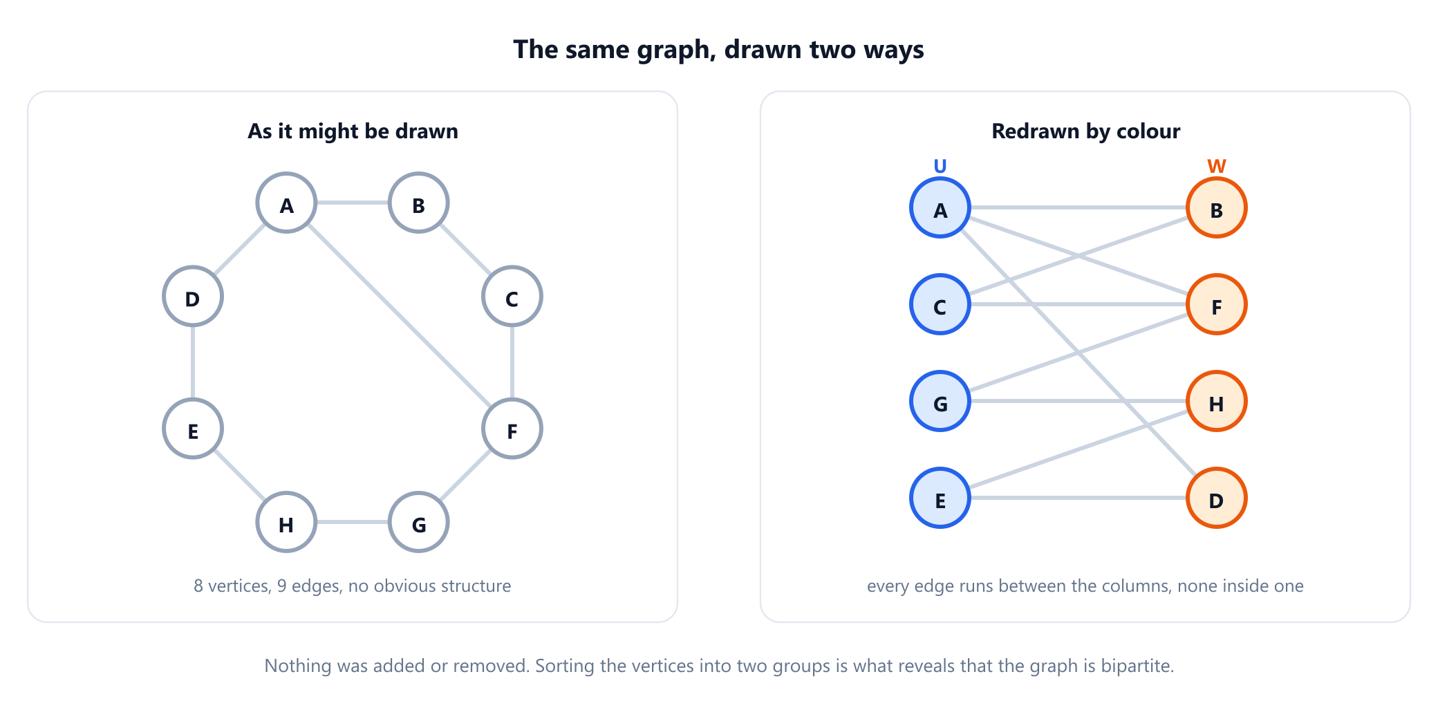
The edge list is short enough to keep in mind:
V = {A, B, C, D, E, F, G, H}
E = {AB, AD, AF, BC, CF, DE, EH, FG, GH}          9 edges

U = {A, C, E, G}      W = {B, D, F, H}             every edge joins U to W
Two edge cases are worth settling at the start. A loop joins a vertex to itself, so both of its ends lie on the same side, and a graph with a loop is never bipartite. Parallel edges change nothing: a second edge between u and v crosses between the sides exactly as the first one did, which is one of the properties the guide to simple graphs and multigraphs lists as unaffected by multiplicity. For a directed graph the question is asked about the underlying undirected graph, since the definition never looks at which way an edge points.
2. Two colours, one bipartition
Paint the vertices of U blue and the vertices of W orange. The definition then says that the two ends of every edge have different colours, which is exactly a proper colouring with two colours. The two descriptions are interchangeable:
A graph is bipartite if and only if it can be properly coloured with two colours. Its chromatic number is then at most 2: exactly 2 if it has at least one edge, and 1 if it has none.
The colouring view explains a fact that the set view hides. In a connected bipartite graph the bipartition is unique, up to swapping the names of the two sides. Colour any one vertex blue and every other vertex is forced: a neighbour must be orange, a neighbour of a neighbour blue, and in general a vertex gets blue exactly when its distance from the starting vertex is even. There is no choice left anywhere. In the running example, {A, C, E, G} against {B, D, F, H} is the only possible split.
A graph with several components behaves differently, because each component can be flipped on its own. With k components there are 2k proper two-colourings and 2k−1 distinct bipartitions, counting every isolated vertex as a component. So "which side is vertex v on?" is a meaningful question inside a component and an arbitrary one across components. Code that stores a single global side for each vertex and then compares sides between unconnected pieces is comparing labels that were chosen independently.
3. Bipartite graphs you have already met
Bipartite graphs are not a special topic tucked away in a later chapter. Several of the most familiar families are bipartite, some of them for reasons that take a moment to see.
- Trees and forests. A tree has no cycles at all, so nothing can go wrong: root it anywhere and colour each vertex by whether its depth is even or odd. Every tree is bipartite, which is one more consequence of the structure developed in trees in graph theory.
- Paths and even cycles. A path alternates colours along its length. A cycle with an even number of vertices does too, and closes up correctly. A cycle with an odd number does not, as the next section proves.
- Grids and chessboards. Colour the square in row
rand columncby the parity ofr + cand you have the chessboard pattern. A step to a neighbouring square changes the parity, so the grid graph is bipartite. A knight's move changes one coordinate by 1 and the other by 2, an odd total, so a knight always lands on the opposite colour and the knight's graph is bipartite as well. - Hypercubes. The cube graph
Qnhas then-bit strings as vertices, with an edge between two strings that differ in exactly one bit. Flipping a bit changes the number of 1s by one, so colouring by the parity of that count works. - Anything built from two kinds of thing. Applicants and jobs, users and products, authors and papers, students and courses. When every edge connects one kind to the other, the graph is bipartite by construction.
The chessboard example has a classic payoff. Remove two diagonally opposite corners from an 8 by 8 board. Can the remaining 62 squares be tiled by 31 dominoes? Each domino covers two neighbouring squares, one of each colour. The two removed corners have the same colour, so the board now has 30 squares of one colour and 32 of the other, and no tiling can exist. In graph terms a domino tiling is a perfect matching in the grid graph, a perfect matching in a bipartite graph needs equal sides, and these sides are unequal. The puzzle was discussed by the philosopher Max Black in 1946 and later made famous by Martin Gardner; it is the shortest argument anywhere for why bipartiteness is worth noticing.
Equally useful are the graphs that are not bipartite. Any graph with a triangle fails, since three mutually adjacent vertices need three colours. That rules out every complete graph Kn with n ≥ 3, and it rules out the seven bridges of Königsberg too: the north bank, the island and the east island form a triangle. The Petersen graph fails without containing any triangle at all, because it is full of 5-cycles.
4. Kőnig's theorem: no odd cycles
Triangles are an obstacle, but they are not the real one. The real obstacle is any cycle of odd length, and it is the only obstacle there is.
Theorem. A graph is bipartite if and only if it contains no cycle of odd length.
The result is due to Dénes Kőnig. Asratian, Denley and Häggkvist trace it to his 1916 paper in Mathematische Annalen, and it appears with proof in his 1936 Theorie der endlichen und unendlichen Graphen, the first textbook of graph theory (the same book discussed in finite and infinite graphs). Both directions of the proof are short, and the second one is an algorithm in disguise.
Bipartite implies no odd cycle. Walk around a cycle v0, v1, …, vk−1 and back to v0. Each step changes the colour, so vi has the same colour as v0 exactly when i is even. The closing edge from vk−1 to v0 joins two different colours only if k − 1 is odd, that is, only if the cycle length k is even.
No odd cycle implies bipartite. Work in one component at a time and pick any root r. Colour each vertex by the parity of its distance from r. Suppose some edge uv joined two vertices of the same colour, so d(u) and d(v) have the same parity. Follow a shortest path from r to u, cross the edge to v, and follow a shortest path from v back to r. That closed walk has length d(u) + d(v) + 1, which is odd.
A closed walk is not yet a cycle, because it may revisit vertices, and this is the step that careless proofs skip. It is repaired by a small lemma: every closed walk of odd length contains a cycle of odd length. If the walk repeats a vertex, split it there into two shorter closed walks; their lengths add up to an odd number, so one of them is odd, and induction on the length finishes the job. The odd cycle contradicts the assumption, so no such edge exists and the distance colouring is proper.
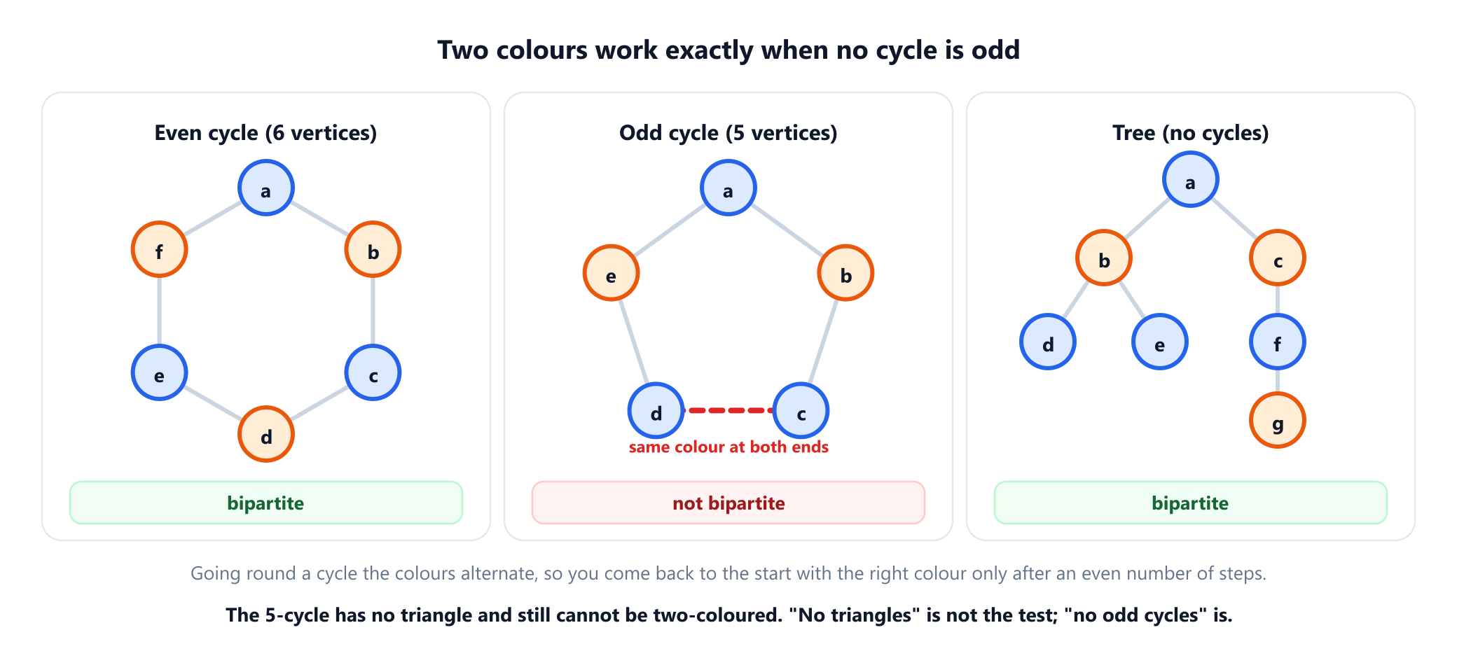
The figure's middle panel carries the trap worth remembering. The 5-cycle is triangle-free and still not bipartite. "No triangles" is a necessary condition and nowhere near a sufficient one. Every odd length counts.
The running example passes. Its cycles have lengths 4 (A, B, C, F), 6 (A, D, E, H, G, F) and 8 (the outer ring), all even. Two easy corollaries are worth having to hand. Deleting edges or vertices can never create an odd cycle, so every subgraph of a bipartite graph is bipartite. Adding a single edge, on the other hand, can destroy the property, as the next section shows.
5. Testing a graph in linear time
The second half of the proof is a procedure. Run a breadth-first search from any vertex, give each newly discovered vertex the colour opposite to its parent, and watch every edge you examine. If some edge ever has the same colour at both ends, the graph is not bipartite. If the search finishes without that happening, the colours are a valid bipartition. Repeat from an uncoloured vertex until every component has been searched.
A good test does more than answer yes or no. It returns a certificate that can be checked independently: the two-colouring when the answer is yes, and an actual odd cycle when the answer is no. The function below does both.
from collections import deque

def bipartite_or_odd_cycle(graph):
    """Return (True, colour) or (False, odd_cycle) for an undirected graph."""
    colour, parent, depth = {}, {}, {}
    for start in graph:                      # every component, not just one
        if start in colour:
            continue
        colour[start], parent[start], depth[start] = 0, None, 0
        queue = deque([start])
        while queue:
            u = queue.popleft()
            for v in graph[u]:
                if v not in colour:          # tree edge: give v the other colour
                    colour[v], parent[v], depth[v] = 1 - colour[u], u, depth[u] + 1
                    queue.append(v)
                elif colour[v] == colour[u]: # same colour on both ends: odd cycle
                    return False, odd_cycle(u, v, parent, depth)
    return True, colour

def odd_cycle(u, v, parent, depth):
    # u and v sit at the same BFS depth; climb until the two paths meet.
    left, right = [u], [v]
    while u != v:
        u, v = parent[u], parent[v]
        left.append(u)
        right.append(v)
    return left + right[-2::-1]              # u ... meet ... v, closed by edge v-u

graph = {
    'A': ['B', 'D', 'F'], 'B': ['A', 'C'], 'C': ['B', 'F'], 'D': ['A', 'E'],
    'E': ['D', 'H'], 'F': ['A', 'C', 'G'], 'G': ['F', 'H'], 'H': ['E', 'G'],
}
ok, colour = bipartite_or_odd_cycle(graph)
print(ok, sorted(v for v in colour if colour[v] == 0))
# True ['A', 'C', 'E', 'G']

graph['C'].append('E'); graph['E'].append('C')   # one extra edge
print(bipartite_or_odd_cycle(graph))
# (False, ['C', 'B', 'A', 'D', 'E'])
The cycle extraction relies on one property of breadth-first search: every edge joins two vertices whose depths differ by at most one. Two vertices with the same colour have depths of the same parity, so a clashing edge always joins two vertices at the same depth. Climbing their parent pointers in lockstep therefore reaches the meeting vertex at the same moment from both sides. If the two climbs take t steps each, the cycle has 2t + 1 edges, which is odd by construction.
Here is what happens on the running example, and then after one extra edge from C to E:
BFS from A        layer 0: A    layer 1: B, D, F    layer 2: C, E, G    layer 3: H
                  every edge joins neighbouring layers   → bipartite, colour 0 = {A, C, E, G}

add edge C-E      C and E both sit in layer 2, so they have the same colour
                  climb from C: C, B, A      climb from E: E, D, A      meet at A
                  odd cycle C, B, A, D, E    5 edges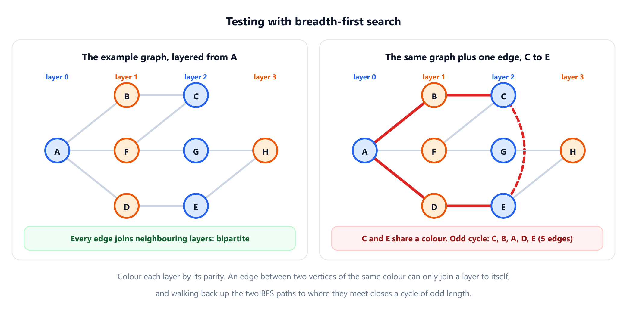
Every vertex is enqueued once and every edge is examined twice, once from each end, so the test runs in O(V + E) time. That is as fast as reading the graph. A depth-first search works just as well in principle, but a recursive DFS in Python hits the default recursion limit of 1,000 on a long path, which is one reason the iterative breadth-first version is the safer default.
One variation is worth knowing. If edges arrive one at a time and you need to know after each insertion whether the graph is still bipartite, rerunning the search is wasteful. A union-find structure that also records each vertex's parity relative to its root answers the question in near-constant amortised time per edge: joining two vertices that already share a root is only allowed if their parities differ.
Watch the two-colouring happen
Build the example graph, run the bipartite check, then add the edge from C to E and watch the search catch the clash and highlight the odd cycle.
Open the bipartite checker6. Complete bipartite graphs and the n²/4 ceiling
The complete bipartite graph Km,n has m vertices on one side, n on the other, and every one of the m × n possible cross edges. It is to bipartite graphs what Kn is to graphs in general: the densest member of the family with given side sizes.
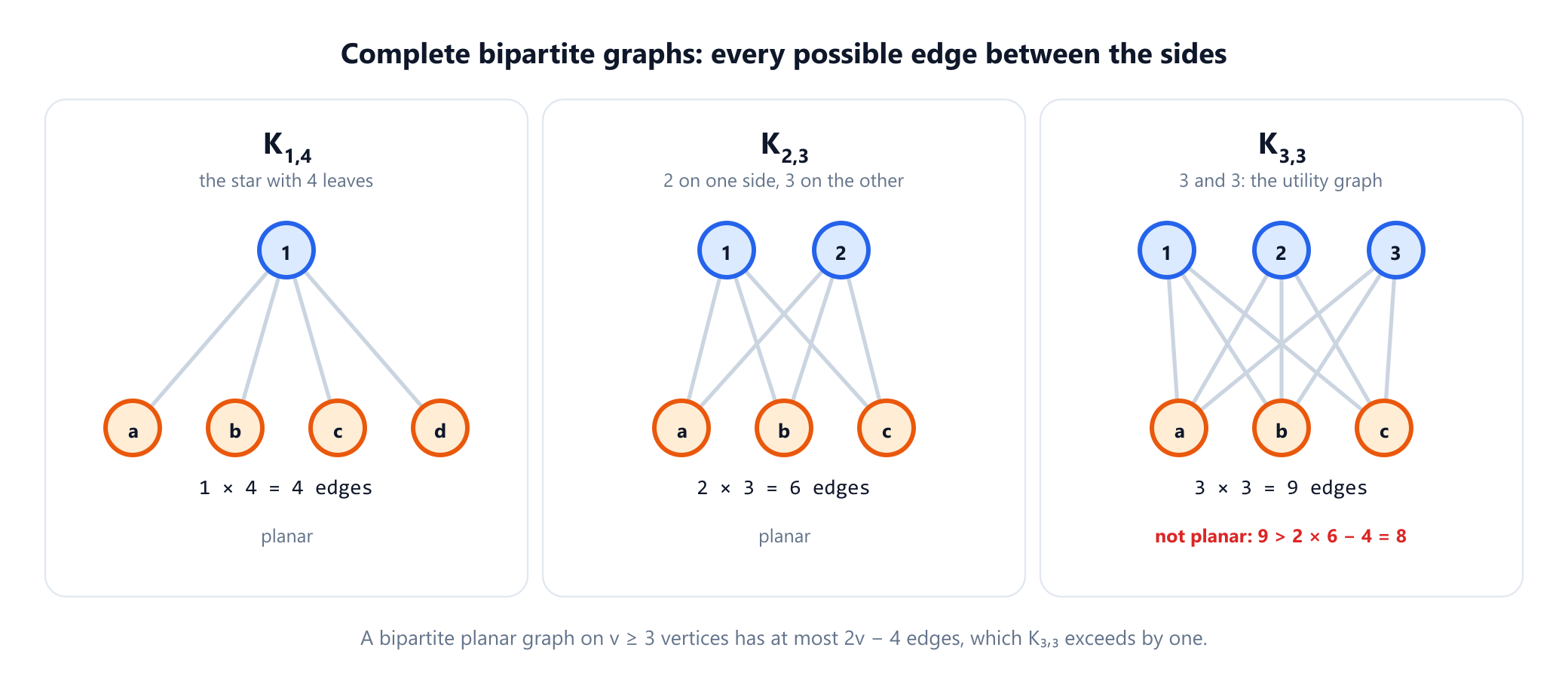
Two members have names of their own. K1,n is the star, a centre joined to n leaves, and it is also a tree. K3,3 is the utility graph of the old puzzle that asks you to connect three houses to three utilities without any lines crossing. The puzzle has no solution: Kuratowski's 1930 theorem says a graph is planar exactly when it contains no subdivision of K5 or K3,3, and K3,3 is one of the two forbidden shapes.
Bipartiteness gives a one-line proof that K3,3 is not planar. In a drawing without crossings, every face is surrounded by a closed walk of edges. A bipartite graph has no triangles, so in a simple connected planar bipartite graph with at least three vertices every face boundary has at least 4 edges. Each edge is counted twice in total across the face boundaries, which gives 4f ≤ 2m. Substituting into Euler's formula v − m + f = 2 yields
m ≤ 2v − 4        for a simple connected planar bipartite graph with v ≥ 3

K3,3:   v = 6,  m = 9,  but 2v − 4 = 8        so no planar drawing exists
A second classical bound concerns density. If one side has k vertices and the other n − k, there are at most k(n − k) edges, and that product is largest when the sides are as equal as possible. So a bipartite graph on n vertices has at most ⌊n²/4⌋ edges, reached by K⌊n/2⌋,⌈n/2⌉. Mantel proved in 1907 that the same ceiling holds for every triangle-free graph, with the balanced complete bipartite graph as the only graph that reaches it. That is a striking pairing with the trap in section 4: triangle-free graphs need not be bipartite, yet the densest triangle-free graph always is. The running example has 9 edges against a ceiling of 16, the edge count of K4,4.
Degrees obey a sharper version of the handshaking lemma. Every edge has exactly one end in each side, so
∑ deg(u) over u in U  =  |E|  =  ∑ deg(w) over w in W

example:   3 + 2 + 2 + 2  =  9  =  2 + 2 + 3 + 2
One quick consequence: if every vertex has the same degree k ≥ 1, then k|U| = k|W|, so a regular bipartite graph always has two sides of equal size. That fact is the first step toward the matching results in the next section.
7. Matchings: why bipartite graphs matter
A matching is a set of edges no two of which share a vertex. In a bipartite graph it is an assignment: each applicant gets at most one job and each job at most one applicant. A matching is perfect when it covers every vertex. Most of the reason bipartite graphs fill textbooks is that matching problems on them are both important and efficiently solvable, and the theory comes with exact certificates.
The first certificate says when everybody on one side can be served.
Hall's theorem (1935). A bipartite graphG = (U, W, E)has a matching that covers every vertex ofUif and only if every subsetS ⊆ Uhas at least|S|neighbours inW.
Read the hypothesis carefully, because it is often misquoted. Hall's condition is about covering one side, not about a perfect matching. The two coincide only when |U| = |W|. The necessity is obvious: if two applicants are each qualified for only one job, and it is the same job, they cannot both be placed. Hall's contribution is that this kind of local shortage is the only thing that can go wrong. A corollary that Kőnig proved in 1916: every k-regular bipartite graph with k ≥ 1 has a perfect matching.
The second certificate proves that a matching cannot be improved. A vertex cover is a set of vertices touching every edge. Each edge of a matching needs its own cover vertex, so no matching is larger than any cover. In bipartite graphs the two meet:
Kőnig–Egerváry theorem (1931). In a bipartite graph, the size of a maximum matching equals the size of a minimum vertex cover.
Outside bipartite graphs this fails at the first opportunity: a triangle has a maximum matching of size 1 and a minimum vertex cover of size 2. In the running example a matching of size 4 exists, and {A, C, E, G} is a vertex cover of size 4, so each certifies that the other is optimal without any search.
Finding a maximum matching uses augmenting paths: a path that starts at an unmatched vertex, alternates between edges outside and inside the matching, and ends at another unmatched vertex. Swapping the two kinds of edge along it grows the matching by one. Berge proved in 1957 that a matching is maximum exactly when no augmenting path exists. On a bipartite graph the search for one is a plain depth-first search, which gives the short method often called Kuhn's algorithm:
def max_matching(left, adj):
    """Kuhn's augmenting-path algorithm. adj maps each left vertex to its right neighbours."""
    match_of = {}                            # right vertex -> left vertex

    def augment(u, seen):
        for v in adj[u]:
            if v in seen:
                continue
            seen.add(v)
            # v is free, or its partner can be moved to another right vertex
            if v not in match_of or augment(match_of[v], seen):
                match_of[v] = u
                return True
        return False

    size = sum(augment(u, set()) for u in left)
    return size, {u: v for v, u in match_of.items()}

adj = {'A': ['B', 'D', 'F'], 'C': ['B', 'F'], 'E': ['D', 'H'], 'G': ['F', 'H']}
size, pairs = max_matching(['A', 'C', 'E', 'G'], adj)
print(size, dict(sorted(pairs.items())))
# 4 {'A': 'D', 'C': 'B', 'E': 'H', 'G': 'F'}
The result is a perfect matching, A–D, C–B, E–H, G–F. It is not the only one: this graph has exactly three perfect matchings. The method runs in O(V · E) time, and like any recursive search in Python it needs an iterative rewrite for very deep graphs. For large instances the standard choice is the Hopcroft–Karp algorithm of 1973, which finds many shortest augmenting paths per phase and runs in O(E √V).
Three related problems are worth knowing by name:
- Weighted assignment. When each edge has a cost and you want the cheapest perfect matching, the Hungarian method of Kuhn (1955) solves it efficiently. The work assignment guide applies it to real staffing decisions.
- Matching as flow. Add a source joined to every vertex of
U, a sink joined from every vertex ofW, give every edge capacity 1, and a maximum flow is a maximum matching. The Kőnig–Egerváry theorem then becomes a special case of max flow equals min cut. - Stable matching. When both sides rank each other, Gale and Shapley (1962) showed that a matching with no pair who would both rather be together always exists, and gave the algorithm that finds it.
8. Edge colouring and timetables
Colouring the edges of a graph so that edges sharing an end get different colours needs at least Δ colours, where Δ is the maximum degree, because the edges at a busiest vertex all clash with each other. For general graphs that is not always enough: a triangle has Δ = 2 and needs 3 colours, and Vizing proved in 1964 that Δ + 1 always suffices for simple graphs. Bipartite graphs never need the extra colour.
Kőnig's edge colouring theorem (1916). The edges of every bipartite graph, multigraphs included, can be coloured with exactly Δ colours.
One way to see it uses Hall's theorem: a bipartite graph can be padded with extra vertices and edges into a Δ-regular bipartite multigraph, which then splits into Δ perfect matchings, one per colour. The running example has Δ = 3, at vertices A and F, and three colours suffice.
This is the theorem behind school timetables. Put teachers on one side and classes on the other, and draw one edge for each lesson that a teacher gives a class in a week, with parallel edges when the same teacher sees the same class several times. A colour is a teaching period, and a proper edge colouring is a timetable in which no teacher and no class is in two places at once. Kőnig's theorem says the number of periods needed equals the heaviest weekly load of any single teacher or class, never more. Real timetables add rooms and preferences that break the clean bipartite structure, which is where the problem turns hard, but the core assignment is a bipartite edge colouring.
9. The matrix view
List the vertices of U first and those of W second, and the adjacency matrix of a bipartite graph falls into blocks. Both diagonal blocks are zero, because there are no edges inside a side:
A  =  [ 0    B ]            B is the |U| × |W| biadjacency matrix
      [ Bᵀ   0 ]

B for the example      B  D  F  H
                   A [ 1  1  1  0 ]
                   C [ 1  0  1  0 ]
                   E [ 0  1  0  1 ]
                   G [ 0  0  1  1 ]
The off-diagonal block B, the biadjacency matrix, holds all the information, so programs store it alone. A user and item ratings table is exactly a weighted biadjacency matrix, which is why recommender systems are naturally graph problems; the trade-offs between storage formats are covered in graph representation.
The block structure leaves a fingerprint on the eigenvalues. If a vector (x, y), split by sides, satisfies A(x, y) = λ(x, y), then (x, −y) satisfies the same equation with −λ. So the spectrum of a bipartite graph is symmetric about zero, and the converse holds too: a graph whose adjacency spectrum is symmetric about zero is bipartite. The running example's eigenvalues are ±2.356, ±1.477, ±1.095 and ±0.262, in perfect pairs. Add the edge from C to E and the pairing breaks, with the largest eigenvalue at 2.592 and the smallest at −2.281. For a connected graph a single number decides it: the graph is bipartite exactly when the negative of its largest eigenvalue is also an eigenvalue. The 5-cycle, for instance, has the eigenvalue 2 but not −2.
Chemists found this before graph theorists named it. In 1940 Coulson and Rushbrooke showed that for alternant hydrocarbons, whose carbon atoms split into two sets with bonds only between the sets, the energy levels of the π-electrons come in pairs placed symmetrically about the middle. That pairing theorem is the bipartite spectrum symmetry, stated for molecules. The wider link between eigenvalues and structure is the subject of spectral graph theory.
10. Where bipartite graphs show up
Bipartite graphs are the honest model whenever a system relates two different kinds of object and never relates two objects of the same kind directly.
| Field | Side U | Side W | An edge means |
|---|---|---|---|
| Staffing and admissions | Workers, students | Shifts, schools | This person can take this slot |
| Recommender systems | Users | Products, films | A purchase, click or rating |
| Collaboration networks | Authors, actors | Papers, films | This person took part in this work |
| Error-correcting codes | Code bits | Parity checks | This bit appears in this check |
| Process modelling | Places (states) | Transitions (events) | An arc of a Petri net |
| Hypergraphs | Vertices | Hyperedges | This vertex belongs to this hyperedge |
Two rows deserve a closer look. In coding theory, Tanner introduced in 1981 the graph now named after him, with code bits on one side and parity checks on the other. Modern low-density parity-check codes, used in Wi-Fi and 5G, are decoded by passing messages back and forth along the edges of exactly this bipartite graph. And any hypergraph, where an edge may join more than two vertices, can be stored without loss as a bipartite incidence graph, which lets ordinary graph algorithms run on it.
The collaboration row hides a common modelling error. Analysts often project a bipartite graph onto one side, joining two authors whenever they share a paper. The projection throws information away. Three authors who wrote one paper together and three authors who wrote three separate papers in pairs produce the same triangle in the projection, although the underlying collaborations are entirely different. Keep the bipartite graph as the source of truth and project only for a specific question.
11. Easy to test, hard to repair
Bipartiteness sits right on the boundary between easy and hard problems, and it is worth seeing exactly where the line falls.
- Two colours: linear time. Section 5 settles it in
O(V + E). - Three colours: NP-complete. Deciding whether a graph can be properly coloured with three colours is one of the standard NP-complete problems catalogued by Garey and Johnson. One more colour turns a breadth-first search into a problem with no known polynomial algorithm, as the graph colouring guide explains.
- Repairing a non-bipartite graph: NP-hard. Deleting the fewest edges to make a graph bipartite is the same as keeping the most edges that cross some split of the vertices, which is the maximum cut problem, one of Karp's 21 NP-complete problems of 1972. Deleting the fewest vertices, the odd cycle transversal problem, is NP-hard as well.
So the odd cycle that the test returns is cheap to find but tells you nothing about the cheapest way to remove all of them. In the running example with the extra edge, deleting C–E restores bipartiteness, but on a large graph with many interlocking odd cycles the minimum repair is genuinely hard to compute.
12. Common mistakes
| Mistake | Why it is wrong | Fix |
|---|---|---|
| Starting the search from one vertex only | A disconnected graph can be bipartite in the searched component and not in another | Loop over all vertices and start a new search from each uncoloured one |
| "It has no triangles, so it is bipartite" | The 5-cycle is triangle-free and not bipartite | Test for odd cycles of every length, which the colouring search does |
| Ignoring loops | A loop puts both ends of an edge on one side | Treat any loop as an immediate "not bipartite" |
| Passing a directed adjacency list | The search only sees edges in one direction and can miss a clash | Symmetrise first: for every arc u → v, add v to u's list and u to v's |
| Comparing sides across components | Each component's colouring was chosen independently | Only compare sides within a component, or fix the sides from the data |
| Calling a greedy matching maximum | Greedy stops at a maximal matching; on the path a–b–c–d picking b–c first gives 1 instead of 2 | Use augmenting paths (Kuhn, Hopcroft–Karp) or a flow formulation |
| Quoting Hall's theorem for perfect matchings | Hall's condition guarantees covering one side; it implies a perfect matching only when the sides are equal | Check |U| = |W| before concluding a perfect matching exists |
13. Glossary
| Term | Meaning |
|---|---|
| Bipartite graph | A graph whose vertices split into two sets with every edge joining the two sets |
| Bipartition | A split (U, W) of the vertex set that witnesses bipartiteness |
| Side, part | One of the two sets of a bipartition; each is an independent set |
| Two-colouring | A proper vertex colouring with two colours; equivalent to a bipartition |
| Odd cycle | A cycle with an odd number of edges; its presence is exactly what prevents bipartiteness |
Complete bipartite graph Km,n | Sides of sizes m and n with all m × n cross edges |
| Biadjacency matrix | The |U| × |W| block of the adjacency matrix recording the cross edges |
| Matching | A set of edges with no shared endpoints |
| Perfect matching | A matching that covers every vertex |
| Vertex cover | A set of vertices touching every edge |
| Augmenting path | An alternating path between two unmatched vertices; flipping it enlarges the matching |
| Odd cycle transversal | A set of vertices whose removal leaves a bipartite graph |
14. Frequently asked questions
What is a bipartite graph?
A bipartite graph is a graph whose vertices can be divided into two disjoint sets so that every edge connects a vertex in one set to a vertex in the other. No edge joins two vertices of the same set. Equivalently, the graph can be coloured with two colours so that the two ends of every edge get different colours.
How do you check if a graph is bipartite?
Run a breadth-first search, give each newly discovered vertex the colour opposite to its parent, and check every edge. If an edge ever joins two vertices of the same colour, the graph is not bipartite, and the two search paths back to their meeting point form an odd cycle that proves it. Restart from every uncoloured vertex so that all components are covered. The test runs in O(V + E) time.
Can a bipartite graph have an odd cycle?
No. Kőnig’s theorem says a graph is bipartite if and only if it has no cycle of odd length. Colours alternate around any cycle, so a cycle can close up properly only after an even number of edges. Having no triangles is not enough: the 5-cycle has no triangle and is still not bipartite.
Is every tree bipartite?
Yes. A tree has no cycles at all, so it has no odd cycle. Concretely, root the tree at any vertex and colour each vertex by whether its depth is even or odd; every edge joins a parent to a child, and their depths differ by exactly one.
What is a complete bipartite graph?
A complete bipartite graph has m vertices on one side, n on the other, and an edge between every vertex of the first side and every vertex of the second, so m times n edges in total. With one vertex on one side it is a star. With three on each side it is the utility graph K₃,₃, which by Kuratowski’s theorem is one of the two graphs whose presence makes a graph non-planar.
Why are bipartite graphs important?
Many real problems relate two different kinds of object, such as workers and shifts, students and schools, users and products, or code bits and parity checks, and those relations form bipartite graphs. On them, matching becomes tractable: Hall’s theorem says when one side can be fully matched, the Kőnig–Egerváry theorem certifies that a matching is maximum, and algorithms such as Hopcroft–Karp and the Hungarian method find maximum and minimum-cost matchings in polynomial time.
15. References
The definitions, theorems and attributions above come from these sources, listed in chronological order.
- Mantel, W. (1907). "Problem 28." Wiskundige Opgaven 10, 60 to 61. The
⌊n²/4⌋bound for triangle-free graphs. - Kőnig, D. (1916). "Über Graphen und ihre Anwendung auf Determinantentheorie und Mengenlehre." Mathematische Annalen 77(4), 453 to 465. The edge colouring theorem for bipartite graphs and perfect matchings in regular bipartite graphs.
- Kuratowski, K. (1930). "Sur le problème des courbes gauches en topologie." Fundamenta Mathematicae 15, 271 to 283. Planarity and the forbidden graphs
K5andK3,3. - Egerváry, J. (1931). "Matrixok kombinatorius tulajdonságairól." Matematikai és Fizikai Lapok 38, 16 to 28.
- Kőnig, D. (1931). "Gráfok és mátrixok." Matematikai és Fizikai Lapok 38, 116 to 119. With Egerváry, the equality of maximum matchings and minimum vertex covers.
- Hall, P. (1935). "On Representatives of Subsets." Journal of the London Mathematical Society 10(1), 26 to 30.
- Kőnig, D. (1936). Theorie der endlichen und unendlichen Graphen. Leipzig: Akademische Verlagsgesellschaft. The first textbook of graph theory, with the odd-cycle characterisation.
- Coulson, C. A. and Rushbrooke, G. S. (1940). "Note on the Method of Molecular Orbitals." Proceedings of the Cambridge Philosophical Society 36(2), 193 to 200. The pairing theorem for alternant hydrocarbons.
- Kuhn, H. W. (1955). "The Hungarian Method for the Assignment Problem." Naval Research Logistics Quarterly 2, 83 to 97.
- Berge, C. (1957). "Two Theorems in Graph Theory." Proceedings of the National Academy of Sciences 43(9), 842 to 844. Augmenting paths characterise maximum matchings.
- Gale, D. and Shapley, L. S. (1962). "College Admissions and the Stability of Marriage." American Mathematical Monthly 69(1), 9 to 15.
- Vizing, V. G. (1964). "On an Estimate of the Chromatic Class of a p-Graph." Diskretnyi Analiz 3, 25 to 30.
- Karp, R. M. (1972). "Reducibility Among Combinatorial Problems." In Complexity of Computer Computations, 85 to 103. New York: Plenum. Maximum cut among the 21 NP-complete problems.
- Hopcroft, J. E. and Karp, R. M. (1973). "An n5/2 Algorithm for Maximum Matchings in Bipartite Graphs." SIAM Journal on Computing 2(4), 225 to 231.
- Garey, M. R. and Johnson, D. S. (1979). Computers and Intractability: A Guide to the Theory of NP-Completeness. San Francisco: W. H. Freeman. Graph 3-colourability as an NP-complete problem.
- Cvetković, D. M., Doob, M. and Sachs, H. (1980). Spectra of Graphs: Theory and Application. New York: Academic Press. Symmetric spectra characterise bipartite graphs.
- Tanner, R. M. (1981). "A Recursive Approach to Low Complexity Codes." IEEE Transactions on Information Theory 27(5), 533 to 547.
- Asratian, A. S., Denley, T. M. J. and Häggkvist, R. (1998). Bipartite Graphs and Their Applications. Cambridge Tracts in Mathematics 131. Cambridge: Cambridge University Press. Source of the 1916 attribution of the odd-cycle theorem.
- Diestel, R. (2017). Graph Theory, 5th edition. Graduate Texts in Mathematics 173. Berlin: Springer.
Two colours or an odd cycle
Draw any graph and let the checker two-colour it. Either every edge ends up crossing between the colours, or it shows you the odd cycle that makes that impossible.
Open the visualizer