
Table of Contents
- 1. Small decisions made every morning
- 2. What a poor assignment costs
- 3. The service day used throughout
- 4. Step one: the day as a bipartite graph
- 5. How the dispatch board does it
- 6. The Hungarian algorithm
- 7. Prices that prove the plan is optimal
- 8. Skills, sick days and Hall's theorem
- 9. Drivers: least total driving or the fairest plan?
- 10. Nurses: preferences and stable matching
- 11. Beyond one person, one job
- 12. What is easy, what is hard
- 13. What the model leaves out
- 14. From whiteboard to optimiser
- 15. Mistakes that quietly cost money
- 16. Frequently asked questions
- 17. References
1. Small decisions made every morning
Every morning, somewhere, a dispatcher decides which technician goes to which job, a nurse manager decides who covers which shift, and a transport planner decides which driver takes which route. Each decision looks small, and each is usually made by hand, from a whiteboard or a spreadsheet, by someone who knows the people involved. Repeated every day across a whole workforce, those decisions set a large share of travel costs, overtime, service quality and staff satisfaction.
The mathematics behind them is one of the oldest and most elegant in operations research. Dénes Kőnig and Jenő Egerváry proved the key theorems in 1931, Philip Hall characterised when a complete assignment exists in 1935, and Harold Kuhn turned their work into the Hungarian algorithm in 1955, naming it after the two Hungarian mathematicians. David Gale and Lloyd Shapley added the theory of stable matching in 1962, work that later earned Shapley and Alvin Roth the 2012 Nobel Memorial Prize in Economic Sciences.
This article follows three real kinds of assignment: field technicians with different skills, delivery drivers who all want a short drive, and nurses with preferences for shifts. Each example is small enough to check every possible plan, so every number below is exact, not estimated.
2. What a poor assignment costs
- Travel. Minutes spent driving are paid but not productive. Counting wages and vehicle costs, each minute of driving is valued here at $1.
- Unfilled work. A job nobody qualified can reach goes to a contractor, rescheduled, or a customer waits. A contractor costs $400 a job here.
- Unfairness. One person with a very long drive, or an unwanted shift every week, costs less on paper than it does in morale, sick leave and turnover.
These figures are illustrative rather than taken from any particular company. The structure is what matters: travel costs add up across a plan, skills restrict who can do what, and fairness and preferences are part of what makes a plan work.
3. The service day used throughout
A heating and utilities service company has nine technicians and eight jobs booked for tomorrow. Jobs need one of three skills: electrical (Jobs 1, 4 and 7), gas (Jobs 2, 5 and 8) and heating and cooling (Jobs 3 and 6). Each technician holds one or two of those qualifications. The table shows the driving time in minutes from each technician's home to each job they are qualified for; a dash means they are not qualified.
| Technician | Skills | Job 1 | Job 2 | Job 3 | Job 4 | Job 5 | Job 6 | Job 7 | Job 8 |
|---|---|---|---|---|---|---|---|---|---|
| Ana | Electrical, heating | 94 | – | 119 | 55 | – | 106 | 75 | – |
| Ben | Gas, electrical | 35 | 93 | – | 75 | 76 | – | 89 | 123 |
| Carla | Electrical | 82 | – | – | 41 | – | – | 44 | – |
| Dev | Heating | – | – | 45 | – | – | 120 | – | – |
| Emil | Gas, heating | – | 91 | 119 | – | 94 | 40 | – | 65 |
| Farah | Electrical, heating | 76 | – | 22 | 87 | – | 127 | 128 | – |
| Gus | Gas, electrical | 43 | 51 | – | 7 | 57 | – | 48 | 46 |
| Hana | Electrical, heating | 37 | – | 103 | 59 | – | 23 | 56 | – |
| Ivo | Heating, electrical | 53 | – | 17 | 80 | – | 105 | 115 | – |
Every job needs exactly one technician, each technician takes at most one job, and one technician will stay free as cover. The goal is the least total driving.
4. Step one: the day as a bipartite graph
Draw technicians on one side and jobs on the other, with an edge for every qualified pair weighted by its driving time. Edges only ever join a technician to a job, never two technicians or two jobs, so the graph is bipartite. A plan is a set of edges in which no technician and no job appears twice, which graph theory calls a matching, and a plan that covers every job is a matching of size eight. The cheapest such matching is the answer to the assignment problem.
Nine technicians could fill eight jobs in 362,880 ways if everyone could do everything. Skills cut that down: only 1,584 plans give every job a qualified technician. That is still far too many to compare on a whiteboard, and a realistic day with 40 technicians has more plans than there are atoms in the Earth.
5. How the dispatch board does it
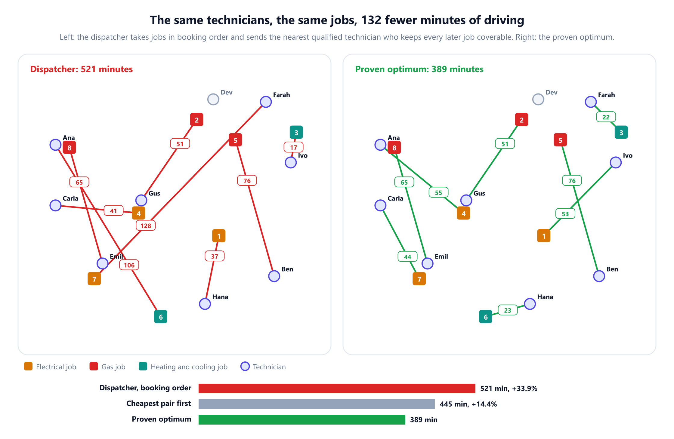
The dispatcher. An experienced dispatcher works through the jobs in booking order and sends the nearest free technician who is qualified. A careful one also keeps enough gas technicians back so that later gas jobs can still be covered, and here that check stops the nearest choice twice. The early jobs get short drives, but by the time Job 7 comes up the only free electrician is Farah, 128 minutes away. The plan totals 521 minutes.
Cheapest pair first. A smarter rule looks at the whole board and repeatedly makes the shortest remaining qualified trip, again without leaving any job uncoverable. It totals 445 minutes, but its early grabs leave Emil a 91-minute drive to Job 2.
The optimum. Checking all 1,584 plans finds one that totals 389 minutes, and it is the only plan that low: the next best costs 406. It sends Ivo to Job 1, Gus to Job 2, Farah to Job 3, Ana to Job 4, Ben to Job 5, Hana to Job 6, Carla to Job 7 and Emil to Job 8, and keeps Dev free. Against the dispatcher it saves 132 minutes a day, about $33,000 a year over 250 working days, and against cheapest pair first it saves 56 minutes a day, about $14,000 a year, for one small team.
Greedy rules fail for the same reason in every assignment problem: a choice that is cheap now can force an expensive choice later, and a rule that never looks ahead cannot see it. The delivery route optimization guide shows the same effect when routes are built one stop at a time.
6. The Hungarian algorithm
Checking every plan works for eight jobs and fails completely for eighty. The Hungarian algorithm finds the optimum without enumeration, in time proportional to n3 for n people, as James Munkres showed in 1957. Its idea is to keep two sets of numbers, one for each side of the graph, and to adjust them until the cheapest plan becomes obvious.
- Reduce. Subtracting the same amount from every travel time in a row, or in a column, does not change which plan is cheapest, because every plan uses exactly one entry from each job's column. Subtract so that every row and column has a zero.
- Look for a complete plan among the zeros. If qualified pairs with reduced time zero form a complete matching, that plan costs nothing extra in the reduced problem, so it is optimal in the original. Finding the largest matching among zeros is a maximum flow question solved with augmenting paths.
- Adjust and repeat. If the zeros cannot cover every job, Kőnig's theorem says they can all be covered by fewer lines than there are jobs. Subtract the smallest uncovered value from the uncovered entries and add it where lines cross. This creates a new zero without making any entry negative, and the algorithm repeats.
Modern implementations, such as the shortest augmenting path method of Jonker and Volgenant (1987), follow the same logic with better bookkeeping, and solve problems with thousands of people in well under a second. Dimitri Bertsekas's auction algorithm (1988) reaches the same optimum by letting jobs raise their prices until every technician is happy with one, which parallelises well.
7. Prices that prove the plan is optimal
The numbers the Hungarian algorithm keeps are more than bookkeeping. At the end, they give every job a price and every technician a value, measured in minutes, with two properties: for every qualified pair, driving time is at least the job's price minus the technician's value, and for every pair in the plan the two are equal.
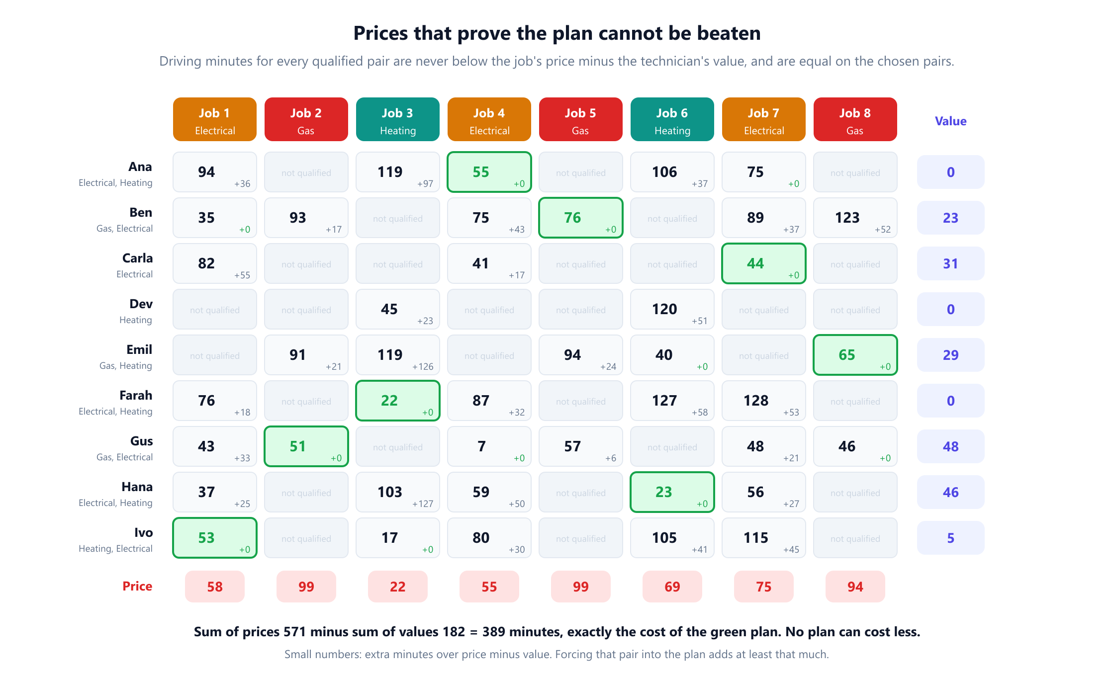
| Job | Job 1 | Job 2 | Job 3 | Job 4 | Job 5 | Job 6 | Job 7 | Job 8 |
|---|---|---|---|---|---|---|---|---|
| Price, minutes | 58 | 99 | 22 | 55 | 99 | 69 | 75 | 94 |
| Technician | Ana | Ben | Carla | Dev | Emil | Farah | Gus | Hana | Ivo |
|---|---|---|---|---|---|---|---|---|---|
| Value, minutes | 0 | 23 | 31 | 0 | 29 | 0 | 48 | 46 | 5 |
The proof takes one line. Any plan gives each job one technician and uses each technician at most once, so its total driving is at least the sum of the eight prices, 571, minus the values of the technicians it uses, which is at most 182. So every plan costs at least 389 minutes, and the green plan costs exactly that. This is linear programming duality, which Egerváry's 1931 theorem anticipated for assignment problems.
The prices also answer practical questions. The extra minutes in each cell are a lower bound on what forcing that pair would cost: sending Dev to Job 3 would add at least 23 minutes to the day. The gas jobs carry the highest prices, 94 and 99, because gas skills are scarce, which is the first hint of the next section.
8. Skills, sick days and Hall's theorem
On Thursday, Emil calls in sick. Eight technicians remain for eight jobs, so on paper everyone can be covered. They cannot. Only Ben and Gus are still qualified for gas, and there are three gas jobs.
Hall's marriage theorem (1935) makes this precise: a complete assignment exists if and only if every group of jobs has at least as many qualified people as jobs. Checking every one of the 255 non-empty groups of jobs finds exactly the failing group here, Jobs 2, 5 and 8, with only two qualified technicians. When a matching algorithm stops short, the same argument hands the planner that group, which says exactly which skill is missing rather than just that the plan failed.
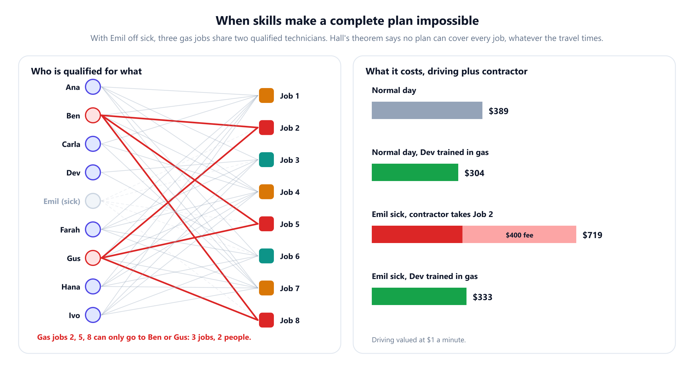
The best response is to send one gas job to a contractor and optimise the rest. Trying each gas job in turn, contracting Job 2 is cheapest: 319 minutes of driving plus the $400 fee, $719 for the day.
Now suppose Dev, who is only qualified for heating, had also been trained in gas. On the sick day the plan would cover every job in-house for $333, saving $386. More surprisingly, the training pays on ordinary days too: with Dev qualified, the normal-day optimum falls from 389 to 304 minutes, because Dev lives 14 minutes from Job 2 and Gus can take Job 4, only 7 minutes away. That is 85 minutes a day, about $21,250 a year, before counting a single sick day. The assignment model turns "who should we cross-train?" into a question with a number attached.
9. Drivers: least total driving or the fairest plan?
A delivery company has nine drivers for seven routes tomorrow, so two drivers will be on standby. Each driver drives from home to the start of a route:
| Driver | Route 1 | Route 2 | Route 3 | Route 4 | Route 5 | Route 6 | Route 7 |
|---|---|---|---|---|---|---|---|
| Ali | 25 | 126 | 47 | 107 | 126 | 127 | 86 |
| Bo | 160 | 24 | 118 | 52 | 104 | 80 | 69 |
| Cy | 44 | 121 | 31 | 95 | 84 | 95 | 76 |
| Dina | 39 | 104 | 10 | 80 | 86 | 91 | 59 |
| Ed | 129 | 10 | 86 | 22 | 81 | 60 | 37 |
| Flo | 162 | 30 | 121 | 57 | 110 | 87 | 73 |
| Gil | 40 | 132 | 40 | 106 | 94 | 106 | 87 |
| Hal | 108 | 36 | 70 | 32 | 89 | 73 | 30 |
| Ines | 102 | 60 | 55 | 33 | 33 | 27 | 29 |
Handing out routes in order, each to the nearest free driver, totals 263 minutes. The assignment with the least total driving, found among all 181,440 plans, totals 222 minutes, but it asks Cy to drive 84 minutes to Route 5 while everyone else drives half an hour or less.
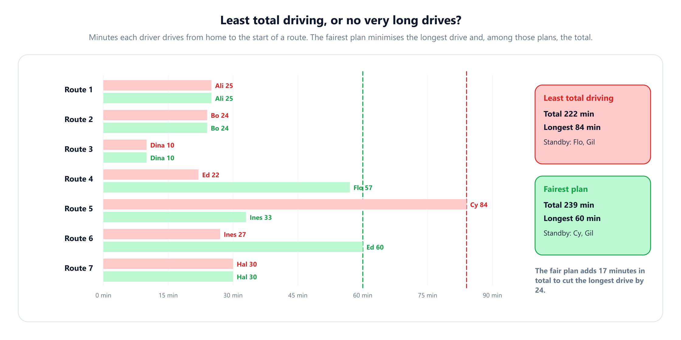
Minimising the longest drive instead is the bottleneck assignment problem, studied by Oliver Gross in 1959. It is solved by asking, for a threshold, whether every route can be covered using only drives no longer than it, which is a matching question, and lowering the threshold until the answer is no. Here the lowest achievable longest drive is 60 minutes, and 60 different plans achieve it. Choosing the one with the least total driving among them gives 239 minutes: 17 minutes, or 7.7%, more than the least total, to take 24 minutes off the worst drive and send Cy to standby.
The fair plan is not fairer by every measure. It has two drives over 45 minutes, 57 and 60, where the least-total plan had one. Fairness has several reasonable definitions: the longest drive, the number of long drives, or the spread between the longest and shortest. Each is a different objective, and the model makes the trade-off visible in minutes instead of leaving it to whoever complains loudest. Over several days, rotating long assignments is another option, and it turns the problem into the kind of roster model used for shift scheduling.
10. Nurses: preferences and stable matching
A hospital unit must fill six shifts with six nurses. Each nurse ranks the shifts, and each shift's manager ranks the nurses by experience and skills:
| Nurse | 1st choice | 2nd | 3rd | 4th | 5th | 6th |
|---|---|---|---|---|---|---|
| Nora | Surgical day | ICU night | Emergency night | Emergency day | ICU day | Children's night |
| Omar | ICU night | Surgical day | Emergency night | Children's night | ICU day | Emergency day |
| Priya | Emergency night | Emergency day | ICU day | ICU night | Surgical day | Children's night |
| Quinn | Emergency night | ICU day | Children's night | Surgical day | ICU night | Emergency day |
| Rosa | Surgical day | Emergency night | Children's night | ICU night | ICU day | Emergency day |
| Sami | Surgical day | Children's night | ICU night | ICU day | Emergency night | Emergency day |
| Shift | Manager's 1st choice | 2nd | 3rd | 4th | 5th | 6th |
|---|---|---|---|---|---|---|
| ICU day | Omar | Nora | Rosa | Priya | Sami | Quinn |
| ICU night | Nora | Omar | Rosa | Priya | Quinn | Sami |
| Emergency day | Omar | Nora | Priya | Rosa | Quinn | Sami |
| Emergency night | Omar | Nora | Priya | Rosa | Sami | Quinn |
| Surgical day | Omar | Nora | Priya | Sami | Rosa | Quinn |
| Children's night | Nora | Omar | Priya | Rosa | Sami | Quinn |
Treating each nurse's rank as a cost, the assignment problem finds the plan with the lowest total rank: 10, with two nurses getting their first choice and the other four their second. It looks ideal. It has a flaw. Priya gets Emergency day, her second choice, while Rosa gets Emergency night. Priya would rather have Emergency night, and that shift's manager would rather have Priya than Rosa. A nurse and a shift who both prefer each other to what the plan gave them form a blocking pair, and plans with blocking pairs tend not to survive contact with reality: swaps get arranged informally, and trust in the process erodes.
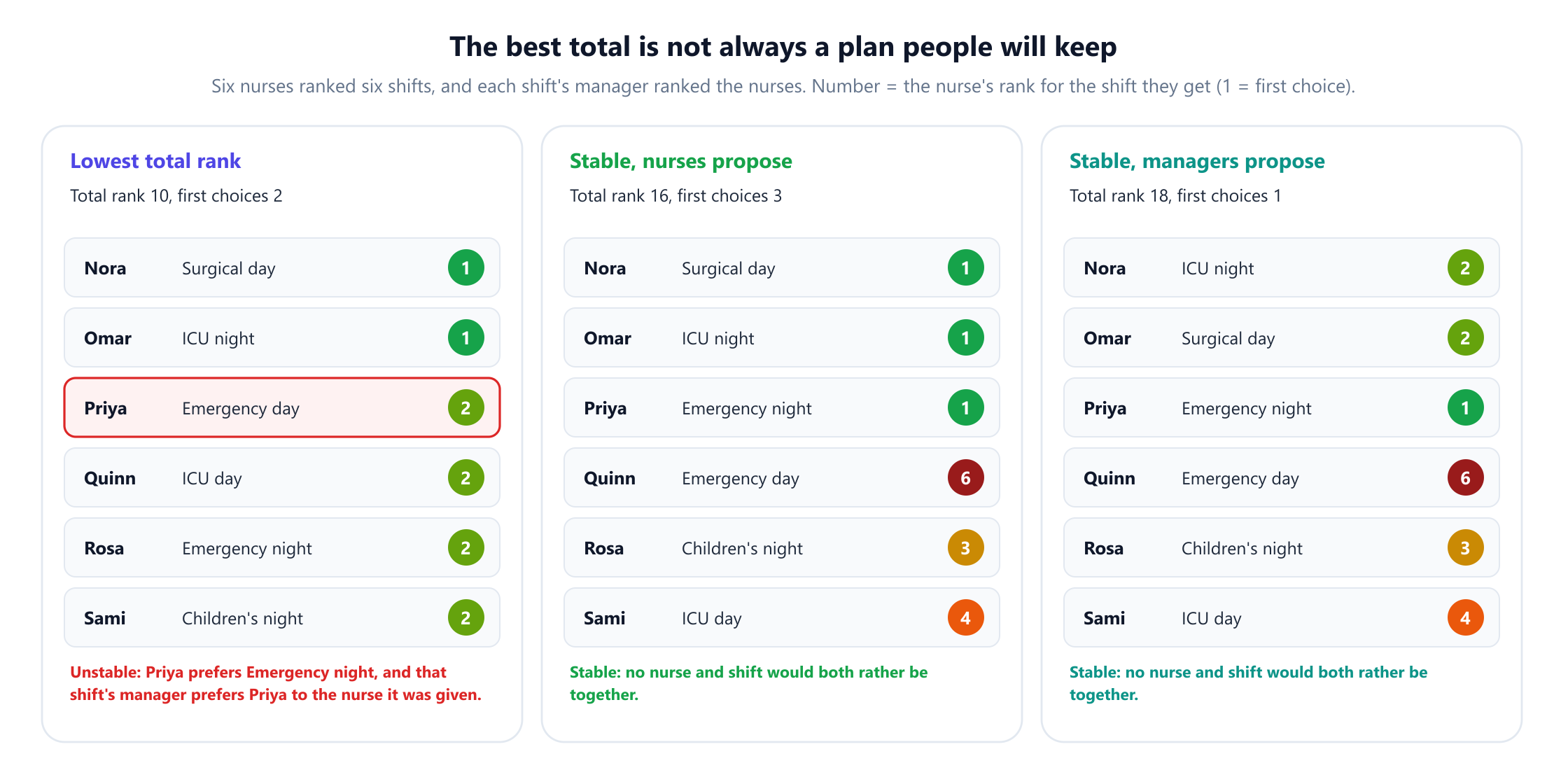
A stable matching has no blocking pairs, and Gale and Shapley proved in 1962 that one always exists. Their deferred acceptance algorithm finds it: each nurse proposes to their favourite shift not yet tried, each manager holds on to the best proposal so far and rejects the rest, and rejected nurses propose again. Here it takes 16 proposals. When nurses propose, the result is the best stable plan for every nurse; when managers propose, it is the best for every manager.
Only two stable plans exist in this unit, with total nurse ranks of 16 and 18. The price of stability is therefore at least 6 rank points, and it falls almost entirely on Quinn, who drops from a second choice to a last choice in both. That is a real dilemma, and there is no formula that settles it. What the model provides is clarity: a manager can choose the lowest total rank and manage the one blocking pair, or choose a stable plan and give Quinn priority next roster. Alvin Roth's redesign of the US medical residency match, with Elliott Peranson in 1999, applied the same deferred acceptance idea to tens of thousands of doctors a year.
11. Beyond one person, one job
- People who take several jobs. If each technician can do up to three jobs and costs still add up, the problem becomes a transportation or minimum-cost flow problem, which is still solved exactly and quickly. Once the order of visits matters, it becomes vehicle routing.
- Jobs of different sizes. When jobs take different amounts of time depending on who does them and each person has limited hours, the problem is the generalised assignment problem. It is NP-hard, and is usually solved with branch and bound on Lagrangian or linear relaxations, following Ross and Soland (1975).
- Three-way assignment. Assigning people to jobs and time slots at once is three-dimensional matching, one of Karp's 21 NP-complete problems (1972).
- Work that arrives during the day. A new emergency job can be inserted greedily or the remaining day re-optimised. Because the Hungarian algorithm is fast, re-solving the whole assignment every time something changes is usually practical.
12. What is easy, what is hard
| Problem | Method | Difficulty |
|---|---|---|
| Can every job be covered by a qualified person? | Bipartite matching (Hopcroft and Karp, 1973) | Polynomial |
| Cheapest one-to-one assignment | Hungarian algorithm (Kuhn, 1955; Munkres, 1957) | Polynomial, O(n3) |
| Assignment minimising the longest single cost | Threshold plus matching (Gross, 1959) | Polynomial |
| A stable matching with two-sided preferences | Deferred acceptance (Gale and Shapley, 1962) | Polynomial, O(n2) |
| Stable matching with the lowest total rank | Irving, Leather and Gusfield (1987) | Polynomial |
| Several jobs per person, additive costs | Transportation or minimum-cost flow | Polynomial |
| Jobs with person-specific sizes and capacities | Generalised assignment problem | NP-hard |
| People, jobs and time slots together | Three-dimensional matching (Karp, 1972) | NP-hard |
The assignment problem is special among combinatorial optimisation problems because its linear programming relaxation always has a whole-number optimum, a consequence of Birkhoff's 1946 theorem on doubly stochastic matrices. Rainer Burkard, Mauro Dell'Amico and Silvano Martello's book Assignment Problems covers the whole family, from these easy cases to the notoriously hard quadratic assignment problem.
13. What the model leaves out
- Job timing. Appointment windows and job durations turn a morning assignment into routing and scheduling for the whole day.
- Uncertain durations and traffic. Travel times vary, so robust plans keep slack and re-optimise during the day.
- Continuity. Customers often prefer the same technician or nurse as last time, a soft preference that can be added as a cost.
- Working time rules. Rest periods, maximum hours and overtime rules link today's assignment to the rest of the week.
- Fairness over time. One day's fair plan can be unfair over a month, so long drives and unpopular shifts should be tracked and balanced across days.
- Strategic behaviour. When people know how preferences are used, they may misreport them. Deferred acceptance is strategy-proof for the proposing side, which is one reason it is used in real matching markets.
14. From whiteboard to optimiser
Build the cost matrix from real data. Travel times come from a routing service or historical GPS data, qualifications from the HR or skills system, and preferences from a simple ranking form. Missing qualifications should be recorded as forbidden pairs, not as very large travel times entered by hand.
Price the current plans first. Take last month's dispatch decisions and compute their total travel against the optimum for the same days. In the example the gap was 132 minutes a day, and a baseline like that is the business case.
Use solid tools. SciPy's linear_sum_assignment and Google OR-Tools' linear sum assignment solver handle the assignment problem directly; minimum-cost flow solvers handle capacities; and mixed integer programming solvers handle side constraints. Stable matching takes a few dozen lines of code.
Agree the objective with the people affected. Least total cost, the longest single drive, preference ranks and stability are all reasonable goals, and they lead to different plans. Showing planners and staff the cost of each option, as sections 9 and 10 do, turns an argument about fairness into a decision.
15. Mistakes that quietly cost money
- Dispatching in booking order. The nearest-technician rule cost 132 minutes a day more than the optimum.
- Trusting a smarter greedy rule. Cheapest pair first still cost 56 minutes a day more.
- Counting heads instead of skills. With Emil sick, eight people could not cover eight jobs, because only two could do gas.
- Treating cross-training as a cost. Training Dev in gas saved 85 minutes on an ordinary day and $386 on a sick day.
- Minimising the total when one person bears it. The least-total plan gave Cy an 84-minute drive; 17 extra minutes in total capped every drive at 60.
- Assuming the best total rank will hold. The lowest-rank nurse plan had a blocking pair; the stable plans cost 6 rank points more.
- Rebuilding the plan by hand after every change. The optimum takes milliseconds to recompute.
16. Frequently asked questions
What is the assignment problem?
+
It is the problem of assigning people to tasks, one task each, so that the total cost, such as travel time, is as small as possible. In graph terms it is finding a minimum-cost perfect matching in a bipartite graph with people on one side and tasks on the other. It can be solved exactly in polynomial time with the Hungarian algorithm, even for thousands of people.
How does the Hungarian algorithm work?
+
It subtracts amounts from rows and columns of the cost matrix, which does not change the best assignment, until a complete assignment can be made using only zero entries. When the zeros are not enough, it adjusts the numbers to create a new zero and repeats. The amounts subtracted become prices and values that prove the final assignment is optimal, and the algorithm runs in time proportional to the cube of the number of people.
Why not send the nearest available worker to each job?
+
Because a short trip now can force a long trip later, when the good options are gone. In the article's example, dispatching jobs in booking order to the nearest qualified technician cost 521 minutes of driving, against 389 for the optimal plan, and choosing the cheapest remaining pair each time still cost 445 minutes.
What does Hall's theorem say about skills?
+
Hall's marriage theorem says every job can be given a different qualified person exactly when every group of jobs has at least as many qualified people as jobs. When coverage fails, the theorem points to the group that is short. In the example, with one gas technician sick, three gas jobs had only two qualified people, so no plan could cover the day even though there were as many people as jobs.
How can work be assigned fairly?
+
One common approach minimises the worst individual cost, such as the longest drive, which is the bottleneck assignment problem, and then minimises the total among plans with that worst case. In the example this cut the longest drive from 84 to 60 minutes for 17 extra minutes of total driving. Other fairness goals, such as limiting the number of long drives or rotating them across days, lead to different plans.
What is a stable matching in nurse scheduling?
+
It is an assignment of nurses to shifts with no nurse and shift that would both prefer each other to what they were given. The Gale-Shapley deferred acceptance algorithm always finds one. A plan with the best total preference rank can be unstable: in the example it had a total rank of 10 but one blocking pair, while the stable plans had total ranks of 16 and 18.
What software solves assignment problems?
+
SciPy's linear_sum_assignment and Google OR-Tools solve the classic assignment problem in a few lines of code. Minimum-cost flow solvers handle people who can take several jobs, and mixed integer programming solvers such as HiGHS or Gurobi handle side constraints like working-time rules. Field service and workforce management systems often include these solvers behind their dispatch screens.
17. References
The foundational papers, surveys and books behind the methods in this article, in chronological order.
- Egerváry, J. (1931). “Mátrixok kombinatorikus tulajdonságairól.” Matematikai és Fizikai Lapok, 38, 16–28.
- Kőnig, D. (1931). “Gráfok és mátrixok.” Matematikai és Fizikai Lapok, 38, 116–119.
- Hall, P. (1935). “On representatives of subsets.” Journal of the London Mathematical Society, 10(1), 26–30.
- Birkhoff, G. (1946). “Tres observaciones sobre el álgebra lineal.” Universidad Nacional de Tucumán, Revista Serie A, 5, 147–151.
- Kuhn, H. W. (1955). “The Hungarian method for the assignment problem.” Naval Research Logistics Quarterly, 2(1–2), 83–97.
- Munkres, J. (1957). “Algorithms for the assignment and transportation problems.” Journal of the Society for Industrial and Applied Mathematics, 5(1), 32–38.
- Gross, O. (1959). The Bottleneck Assignment Problem. Paper P-1630. Santa Monica: RAND Corporation.
- Gale, D. and Shapley, L. S. (1962). “College admissions and the stability of marriage.” American Mathematical Monthly, 69(1), 9–15.
- Karp, R. M. (1972). “Reducibility among combinatorial problems.” In R. E. Miller and J. W. Thatcher (eds.), Complexity of Computer Computations, 85–103. New York: Plenum.
- Hopcroft, J. E. and Karp, R. M. (1973). “An n5/2 algorithm for maximum matchings in bipartite graphs.” SIAM Journal on Computing, 2(4), 225–231.
- Ross, G. T. and Soland, R. M. (1975). “A branch and bound algorithm for the generalized assignment problem.” Mathematical Programming, 8(1), 91–103.
- Jonker, R. and Volgenant, A. (1987). “A shortest augmenting path algorithm for dense and sparse linear assignment problems.” Computing, 38(4), 325–340.
- Irving, R. W., Leather, P. and Gusfield, D. (1987). “An efficient algorithm for the ‘optimal’ stable marriage.” Journal of the ACM, 34(3), 532–543.
- Bertsekas, D. P. (1988). “The auction algorithm: a distributed relaxation method for the assignment problem.” Annals of Operations Research, 14(1), 105–123.
- Roth, A. E. and Peranson, E. (1999). “The redesign of the matching market for American physicians: some engineering aspects of economic design.” American Economic Review, 89(4), 748–780.
- Burke, E. K., De Causmaecker, P., Vanden Berghe, G. and Van Landeghem, H. (2004). “The state of the art of nurse rostering.” Journal of Scheduling, 7(6), 441–499.
- Burkard, R., Dell'Amico, M. and Martello, S. (2012). Assignment Problems, revised reprint. Philadelphia: SIAM.