
Table of Contents
- 1. Why routing is where fleet money is won or lost
- 2. What a route actually costs
- 3. Step one: from a road map to a distance matrix
- 4. The delivery day used throughout
- 5. How routes get planned without optimisation
- 6. The Clarke and Wright savings algorithm
- 7. Local search: repairing a plan one move at a time
- 8. Five plans for the same day, priced
- 9. Fleet size: the van nobody questions
- 10. Delivery windows: pricing a promise
- 11. Beyond twelve stops: how real solvers work
- 12. What the model leaves out
- 13. Running a route optimisation project
- 14. Mistakes that quietly cost money
- 15. Frequently asked questions
- 16. References
1. Why routing is where fleet money is won or lost
A delivery fleet spends money in three places: the vehicles themselves, the fuel and wear of driving them, and the hours of the people behind the wheel. Every one of those costs is decided, every morning, by a plan that says which van visits which customers and in what order. The plan is usually made quickly, by an experienced dispatcher, and it is usually reasonable. The question this article answers is how far "reasonable" is from "best", in money, and which algorithms close the gap.
The problem has a name and a long history. Dantzig and Ramser posed it in 1959 as "the truck dispatching problem", motivated by delivering gasoline to service stations, and it has been known since as the vehicle routing problem. Five years later Clarke and Wright published the savings algorithm that is still built into commercial planning software. Laporte's retrospective Fifty Years of Vehicle Routing (2009) traces how the field grew from those two papers into one of the most studied problems in operations research, and the problem is used in practice at every scale, from a bakery with three vans to parcel carriers with tens of thousands of routes.
What makes it a graph problem is simple. Depots, customers and road intersections are vertices, streets are arcs, and a route is a walk through the graph that starts and ends at the depot. Once the day is written down that way, the planning questions become precise: shortest paths build the distance table, combinatorial search builds the routes, and the answer can be priced and compared rather than argued about.
This article takes one realistic delivery day, twelve customers and a small fleet of vans on a road network with a river and one-way streets, and plans it five ways. The last plan is not a heuristic: it comes from an exhaustive search that checks every possible grouping of customers, so every other plan can be measured against a proven optimum. All the numbers below were computed by solving the model, not estimated.
2. What a route actually costs
"Shortest route" is the phrase everyone uses and almost never the thing a business should minimise. A van on the road incurs three separate costs, and they scale with three different things.
| Cost | Grows with | Value used in this article |
|---|---|---|
| Running cost: fuel, tyres, maintenance | Kilometres driven | $0.60 per km |
| Driver cost | Hours on shift, driving and serving | $28 per hour, at 30 km/h in town, 6 minutes per stop |
| Vehicle cost: lease, insurance, depreciation | Vans used that day | $90 per van per day |
These values are illustrative rather than taken from any particular company, but their proportions are typical of urban delivery, and the conclusions below depend on the proportions, not the exact figures. Your own numbers belong in your own model.
Two consequences follow immediately, and both surprise people. First, at 30 km/h the driver's wage adds about $0.93 to every kilometre, so a kilometre really costs about $1.53, not $0.60. Planning tools that price only fuel undervalue distance by more than half. Second, one van's daily fixed cost of $90 buys about 59 km of driving. So a plan that is 20 km shorter but needs one more van is not a better plan; it is roughly $59 a day worse. As section 8 shows, the classic Clarke and Wright algorithm makes exactly that trade on this day, and the dispatcher's plan pays for the same unnecessary van.
So the objective for the rest of this article is the full daily cost: running cost plus driver cost plus one fixed charge per van used. Distance still matters, but it is one line on the bill, not the bill.
3. Step one: from a road map to a distance matrix
Before any route can be planned, the planner needs to know the travel distance between every pair of places that matter: the depot and each customer. That table, the distance matrix, is the only input a route optimiser actually reads. It is also the step most often done badly.
The road network is a directed graph: intersections are vertices and each drivable direction of a street is an arc with a length. The distance from A to B is the length of the shortest path, and Dijkstra's algorithm (1959) computes it from one origin to every destination at once. Running it once from the depot and once from each customer fills the whole matrix: thirteen runs for thirteen places.
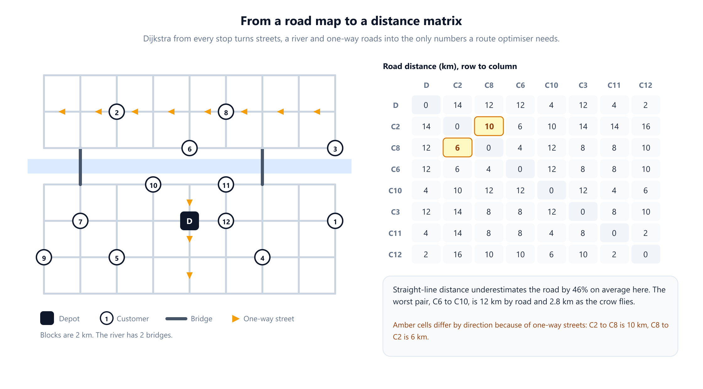
Two features of this network show why the step cannot be skipped by measuring straight lines on a map.
Barriers make detours. The river has two bridges. Customer C6 sits just north of the river and C10 just south of it, 2.8 km apart as the crow flies, but the shortest drive between them is 12 km, more than four times longer. Across all pairs of places in this example, road distance is on average 46% longer than straight-line distance. A plan built on straight lines could treat C6 and C10 as neighbours and send a van on a long detour.
One-way streets break symmetry. Driving from C2 to C8 takes 10 km, while driving from C8 to C2 takes 6 km, because a westbound one-way street runs past both. The matrix is therefore not symmetric, and the order in which a van visits two customers changes the distance, not just the timing. This matters later: some improvement moves that are safe on symmetric data, such as reversing part of a route, have to be re-costed in full on real roads.
In practice nobody runs Dijkstra on a hand-drawn grid. Matrices come from a routing engine over real map data, such as the open-source OSRM or a commercial mapping API, often with travel times that vary by time of day. But the engine is doing exactly this computation, at scale, with faster variants of the same shortest path algorithms described in shortest path algorithms.
4. The delivery day used throughout
The depot sits south of the river. Twelve customers have placed orders today, measured in crates, and each van carries at most 60 crates. Every van leaves the depot at 08:00 and returns when its last delivery is done.
| Customer | Crates | Customer | Crates |
|---|---|---|---|
| C1 | 22 | C7 | 14 |
| C2 | 21 | C8 | 12 |
| C3 | 9 | C9 | 12 |
| C4 | 14 | C10 | 8 |
| C5 | 8 | C11 | 14 |
| C6 | 21 | C12 | 10 |
Total demand is 165 crates. Since 165 divided by 60 is 2.75, no plan can use fewer than three vans, and three vans leave only 15 crates of slack across the whole fleet. That tightness is deliberate and realistic: it is exactly the situation in which the difference between packing well and packing badly is a whole extra vehicle.
In the graph language of the rest of the article, this is the capacitated vehicle routing problem: find a set of routes, each starting and ending at the depot, that together visit every customer exactly once, never exceed a van's capacity, and minimise the total cost from section 2. It is NP-hard, as Lenstra and Rinnooy Kan showed in 1981, because it contains the travelling salesperson problem as the special case of one van with unlimited capacity. With twelve customers it is still small enough to solve exactly, which is the point: it gives us an answer key.
5. How routes get planned without optimisation
Two common manual methods make a fair baseline, because both are what a sensible person does without software.
The sweep. Imagine a clock hand pivoting at the depot. Sweep it round, adding customers to the current van in the order the hand meets them, and start a new van as soon as the next customer would not fit. Then let each driver go to the nearest unvisited stop, then the nearest after that. This is close to the sweep method that Gillett and Miller formalised in 1974, and it is how many dispatchers think about territory: by direction.
On this day the sweep produces four vans. The first three vans fill up in the order the clock hand meets the customers, and the last customer in the sweep, C7 with 14 crates, does not fit in the third van, so a fourth van makes a 12 km round trip for a single delivery. The plan covers 116 km and costs $571.47 for the day.
Nearest neighbour. The second method ignores direction: a van drives to the closest customer it can still carry, then the closest one after that, and heads home when nothing else fits. This plan manages with three vans, drives 108 km and costs $469.20.
Neither method is foolish, and the second is already quite good. Their weakness is that both decide one step at a time and never revisit a decision. The sweep does not notice that its fourth van exists only because of the order in which it met the customers, and nearest neighbour does not notice that the nearest stop now can force an expensive trip later. Algorithms that look at the whole day at once do better, as the next two sections show.
6. The Clarke and Wright savings algorithm
Clarke and Wright's 1964 algorithm starts from the most wasteful plan imaginable, one van per customer, each driving out and back, and then merges routes in the order that saves the most distance.
The key quantity is the saving of serving customer j straight after customer i on one van instead of on two separate trips. Two trips drive i back to the depot and then out to j; one merged trip drives straight from i to j. So the saving is:
saving(i, j) = d(i, depot) + d(depot, j) - d(i, j)Compute the saving for every ordered pair, sort from largest to smallest, and work down the list. Whenever i is the last stop of one route and j is the first stop of another, and the combined load fits in a van, merge the two routes. Because this road network has one-way streets, the formula is applied to ordered pairs: joining "...C2" to "C8..." is not worth the same as joining "...C8" to "C2...".
On this day the largest savings are 20 km, for joining C2 with C6 and C6 with C8, customers that sit close together north of the river, far from the depot. The algorithm merges those first, then works outwards. It finishes with 104 km of driving, less than either manual plan, and costs $553.07. That is worse than nearest neighbour, despite the shorter distance, because it too uses four vans.
The fourth van is the textbook weakness of savings, and it is worth understanding exactly. The algorithm left customer C12 on a van of its own, a 4 km round trip, because C12 sits right next to the depot. Shortest paths obey the triangle inequality, so no merge involving C12 can ever save more than C12's own round trip: merging it with anything saves at most 4 km. Customers near the depot therefore tend to sink to the bottom of the savings list. On this day two of the other routes were too full by then to take C12's 10 crates, and the one route with room to spare, C5-C9-C7-C10, offered a saving of exactly zero at both of its ends, so the algorithm never merged it. Savings minimises kilometres, and this day shows that saving kilometres is not the same as saving money.
7. Local search: repairing a plan one move at a time
Construction algorithms such as the sweep, nearest neighbour and savings build a plan once. Local search takes a finished plan and keeps improving it with small edits, accepting any edit that lowers the total cost, until no edit helps. Three moves do most of the work in practice:
- Relocate: take one customer out of its route and insert it somewhere else, in the same route or a different one. If that empties a route, the van is no longer needed.
- Swap: exchange two customers between two routes.
- 2-opt: reverse a stretch of a single route, which removes two road connections and adds two others. Croes introduced this move for the travelling salesperson problem in 1958, Lin generalised it in 1965, and moving a short run of stops elsewhere in the route is Or's 1976 refinement.
Each move is evaluated by re-costing the affected routes, and on asymmetric roads that re-costing must be done in full: reversing a stretch of a route changes its length when a one-way street is involved, so the shortcut formulas used on symmetric data give wrong answers here.
Starting from the savings plan, local search needs only two moves. The first relocates C12 from its lonely van into another route that has room for its 10 crates. C12 lies on roads that route already drives, so the move adds no distance at all and simply removes a van: the daily cost falls from $553.07 to $463.07, exactly one van's $90. The second is a 2-opt move inside one route, which brings the cost down to $456.93. No further single move improves the plan.
That final figure turns out to be the proven optimum, as the next section confirms. Local search does not always get there. Started from the dispatcher's sweep plan instead, the same moves also remove the extra van, but they stop at $463.07, 1.3% above optimal, in a plan where no single relocate, swap or 2-opt move helps even though a better plan exists. This is called a local optimum, and escaping local optima is precisely what the metaheuristics of section 11 are designed to do.
8. Five plans for the same day, priced
To know how good a plan is, you need the best plan to compare against. For twelve customers it can be found exactly. Of the 4,095 possible non-empty groups of customers, 805 fit in one van. For each of those, a dynamic program in the style of Held and Karp (1962) finds the cheapest order to visit the group, and a second dynamic program then chooses the combination of groups that covers every customer exactly once at the lowest total cost. This is the set-partitioning view of vehicle routing that Balinski and Quandt described in 1964, solved here by brute force because the instance is small.
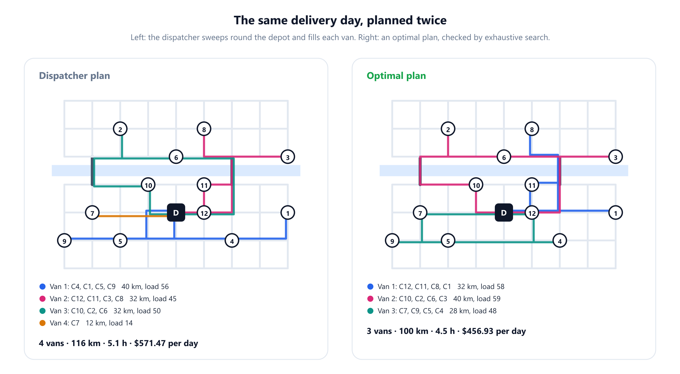
The optimum for this day costs $456.93, with three vans and 100 km. It is not unique: the plan local search found in section 7 and the plan the exhaustive search returned use different routes, yet both reach exactly this cost, which is common in routing, where many arrangements tie. Here is every method on one table.
| Method | Vans | Distance | Driver hours | Daily cost | Above optimum |
|---|---|---|---|---|---|
| Dispatcher sweep | 4 | 116 km | 5.1 | $571.47 | +25.1% |
| Nearest neighbour | 3 | 108 km | 4.8 | $469.20 | +2.7% |
| Clarke and Wright savings | 4 | 104 km | 4.7 | $553.07 | +21.0% |
| Savings, then local search | 3 | 100 km | 4.5 | $456.93 | 0% |
| Proven optimum | 3 | 100 km | 4.5 | $456.93 | 0% |
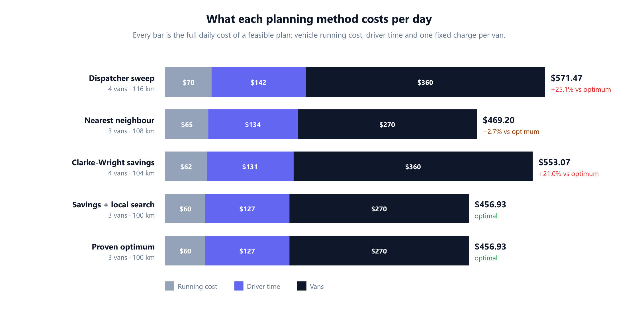
Read the table by columns and three lessons stand out.
The biggest saving is a vehicle, not a kilometre. The optimal plan is $114.54 a day cheaper than the dispatcher's, a 20% reduction. Of that, $90 is the fourth van. The remaining $24.54 comes from 16 fewer kilometres and the driver time they take.
Shorter is not cheaper. Savings drives 4 km less than nearest neighbour and costs $83.87 more. Any planning tool that reports only kilometres would rank these two plans the wrong way round.
Construction plus improvement is a strong recipe. Neither the savings algorithm nor local search alone is remarkable, but together they reached the optimum in two moves. That pairing, a quick construction followed by improvement, is the backbone of most practical routing software, usually with a metaheuristic on top to escape local optima.
Over a working year the gap compounds. If every delivery day looked like this one, the difference between the dispatcher's plan and the optimum over 250 working days would be about $28,600 for a three-van operation. Real days vary, and real savings depend on how good the current planning already is, but the order of magnitude is why fleets invest in optimisation.
9. Fleet size: the van nobody questions
Two of the five methods sent out a fourth van, and in both cases nobody decided to: it was a side effect of the order in which customers were considered. Fleet size is usually treated as fixed, and it deserves to be an output of the plan instead.
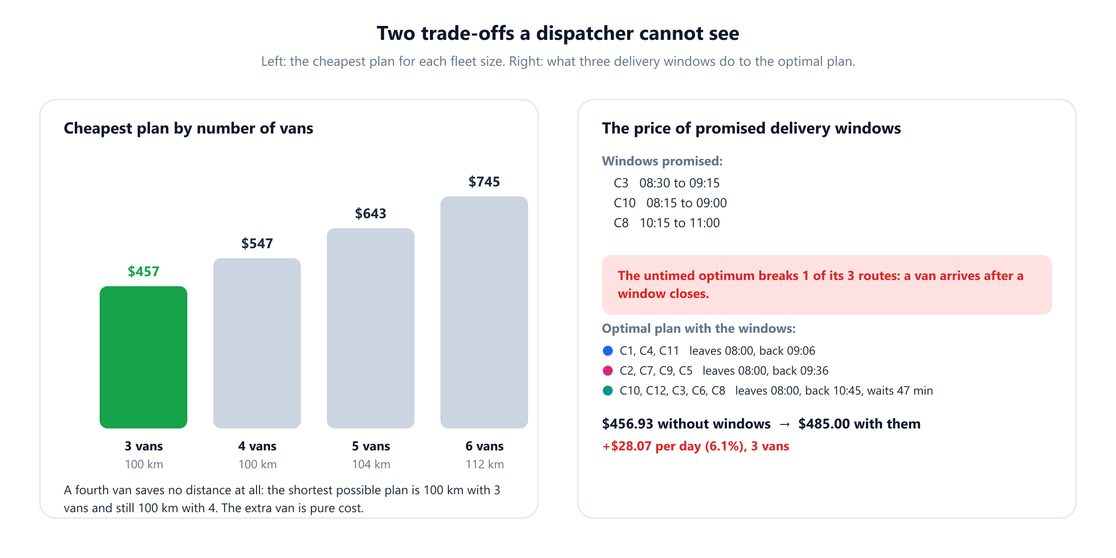
Solving the day exactly for each possible fleet size gives a sharp answer. The cheapest three-van plan costs $456.93. The cheapest four-van plan costs $546.93, exactly $90 more, because the minimum total distance with four vans is 100 km, the same as with three. Splitting the customers across one more van buys no shorter driving at all on this network, so the extra vehicle is pure cost.
That will not always be true. When customers are spread far apart, or when routes are long enough that driver overtime starts, an extra van can pay for itself by shortening every route. The point is that this is a calculation, not a judgement call, and it should be run whenever order volumes change. The breakeven rule from section 2 gives a quick check: an extra van is worth it only if it removes more than about 59 km of driving, at these cost rates.
The same reasoning applies over a longer horizon. The number of vans a business leases is a strategic decision, and the right way to make it is to solve many representative days with different fleet sizes and look at the whole distribution of costs, including the busiest days, rather than to size the fleet for an average day.
10. Delivery windows: pricing a promise
Customers increasingly ask for, and are sold, delivery windows. Each one is a constraint on the plan, and each constraint has a price. Few businesses ever measure it.
Suppose three customers are promised 45-minute windows: C10 between 08:15 and 09:00, C3 between 08:30 and 09:15, and C8 between 10:15 and 11:00. A van that arrives early waits, with the driver paid for the wait; a van that would arrive late is not allowed. This is the vehicle routing problem with time windows, whose standard benchmark instances were published by Solomon in 1987.
The optimal plan from section 8 no longer works. One of its vans serves C10, then C2 and C6 north of the river, and reaches C3 at 09:21, six minutes after the window closes. Re-solving the day exactly with the windows gives a new optimum of $485.00, still with three vans but with a longer day for one of them. The promise costs $28.07 per day, 6.1% more than the unconstrained plan.
Where that money goes is the instructive part. The new plan drives 104 km instead of 100, which accounts for about $6 of the increase. The other $21.93 is waiting: one van arrives early twice, and its driver waits 47 minutes in total, 7 minutes for C10's window to open and 40 minutes for C8's. Nothing about the road network changed. The cost is entirely the promise.
This is the kind of number commercial teams rarely see and should. A narrow morning slot offered free of charge to one customer can cost more per day than that customer's margin, while widening a window from 45 minutes to two hours might cost nothing at all. Measuring the price of route duration and waiting properly is its own research topic; Savelsbergh's 1992 paper on minimising route duration under time windows is a classic treatment of the waiting-time effect seen here.
11. Beyond twelve stops: how real solvers work
Twelve customers could be solved exhaustively in well under a second. Real fleets are larger, and the growth is brutal. A single van leaving the depot to visit just twelve stops already has 12!/2, almost 240 million, distinct round trips when distances are symmetric, and every customer added multiplies that count again. With a hundred customers and a fleet to divide them among, enumeration is impossible, and the question becomes how close to optimal a method can get in the minutes a morning allows.
Modern methods fall into two families.
Metaheuristics run local search but refuse to stop at the first local optimum. Tabu search temporarily forbids undoing recent moves so the search can climb out of a valley; Gendreau, Hertz and Laporte's 1994 algorithm was an influential early success for vehicle routing. Large neighbourhood search, introduced for routing by Shaw in 1998, destroys a sizeable part of the plan, for example all customers in one district, and rebuilds it; Ropke and Pisinger's 2006 adaptive version learns which destroy and repair rules work best as it runs. Hybrid genetic search, developed by Vidal and colleagues from 2012 onwards and released as open source in 2022, combines a population of plans with intensive local search and is among the strongest published methods for the capacitated problem.
Exact methods prove optimality, or at least bound the gap. The leading approach is branch-cut-and-price: a column-generation formulation in which each column is a feasible route, strengthened with cutting planes and embedded in branch and bound. Pecin and colleagues' 2017 algorithm solved benchmark instances with a few hundred customers to proven optimality. Uchoa and colleagues published a harder benchmark set the same year, with instances from 100 to 1,000 customers, partly because the older sets had become too easy to separate the best methods.
For a business the practical conclusion is reassuring. You do not need the exact methods: well-implemented metaheuristics routinely land within a small percentage of the best known solutions on benchmark instances, and the lower bounds from exact methods tell researchers how small that gap really is. The larger gap in most fleets is not between a good metaheuristic and the optimum; it is between the current manual plan and any good algorithm, which is the gap this article measured.
12. What the model leaves out
The delivery day above is a clean model, and a real deployment has to add the features that clean models leave out. Each has a well-studied extension.
- Travel times change during the day. A route that is quick at 06:00 can be slow at 08:30. Time-dependent vehicle routing, formulated by Malandraki and Daskin in 1992, uses travel times that depend on departure time, which also breaks the assumption that reversing a route keeps its duration.
- Orders arrive during the day. Same-day and on-demand delivery require dynamic routing: re-optimising the remaining plan as new orders and delays arrive, without disrupting drivers already on the road.
- Drivers have rules. Legal driving hours, mandatory breaks and shift lengths turn into constraints on route duration and can change which plans are feasible. Deciding which drivers work which days is a rostering problem of its own, covered in employee shift scheduling.
- Vehicles differ. Mixed fleets with different capacities, costs, and access restrictions such as low-emission zones or weight limits change the cost of each route by vehicle.
- Stops are not points. Parking, walking to the door, stairs and failed deliveries all affect service time, which is often the least accurate number in the data and one of the most influential.
- Some routes carry goods both ways. Returns, pickups and deliveries on the same route give the pickup and delivery problem, where the order of stops is constrained by what is on board.
None of these changes the core picture: a graph of places, a cost for every route, and a search for the cheapest set of routes. They change the constraints on what a route may be and the data needed to price it. For how routing fits into the wider network of plants, warehouses and flows upstream of the van, see graph theory in supply chain optimization.
13. Running a route optimisation project
The algorithms are the well-understood part. Projects succeed or fail on four other things.
Get the data right first. Accurate customer locations, realistic service times per stop, vehicle capacities in the unit that actually binds (weight, volume or pallets), and cost rates agreed with finance. A plan optimised against wrong service times will be confidently infeasible by mid-morning, and drivers will stop trusting it within a week.
Measure the baseline honestly. Price last month's actual routes with the same cost model before optimising anything. Without that baseline, there is no way to show what the project earned, and the comparisons in section 8 are only meaningful because every plan was priced the same way.
Choose tools that match the scale. For many fleets an existing solver is the right starting point. Google OR-Tools includes a vehicle routing solver with capacities, time windows and custom costs; VROOM is an open-source optimisation engine designed to work with routing engines such as OSRM; and Helsgaun's LKH-3 extends the Lin-Kernighan heuristic to many routing variants. Commercial platforms add driver apps, live tracking and re-planning. Building from scratch is justified when the constraints are genuinely unusual.
Roll out with the dispatchers, not around them. Experienced dispatchers know things the data does not: which customer's loading bay is blocked on Tuesdays, which street floods. The most effective deployments treat the optimiser as a proposal the dispatcher can adjust, and feed the adjustments back into the data. Large-scale successes such as UPS's ORION system, described by Holland and colleagues in 2017, took years of exactly this kind of iteration between algorithm, data and the people on the road.
14. Mistakes that quietly cost money
These are the errors that produce plans which look fine and cost more than they should.
- Minimising distance instead of cost. As section 8 showed, the shortest plan here used a van too many. Price vans and driver hours, not only kilometres.
- Using straight-line distances. On this network they were 46% short on average and more than four times short for one pair. Use road distances from a routing engine.
- Assuming distances are symmetric. One-way streets and turn restrictions make A to B differ from B to A. A symmetric matrix silently gets the order of stops wrong.
- Treating fleet size as fixed. The fourth van in two of our plans was a side effect, not a decision. Let the optimiser decide how many vehicles to use.
- Giving away delivery windows. Three narrow windows added 6.1% to this day's cost. Know the price of a promise before offering it.
- Trusting a construction heuristic alone. Savings is a good start and was 21% above optimal on its own here. Always follow construction with improvement.
- Inventing service times. A guess of two minutes per stop when reality is six makes every route infeasible. Measure them from past deliveries.
- Optimising once. Orders, traffic and fleet change. A plan that was optimal in March is not optimal in December; routing should be re-solved for every planning period.
15. Frequently asked questions
What is delivery route optimization?
+
It is the process of deciding which vehicle serves which customers, and in what order, so that every delivery is made within the vehicles' capacities and any time windows at the lowest total cost. Mathematically it is the vehicle routing problem: customers and the depot are vertices of a graph, road distances come from shortest paths, and the solver searches for the cheapest set of routes that starts and ends at the depot.
How much can route optimization save?
+
It depends on how good the current planning is, so the only honest answer is to price your current routes and an optimised plan with the same cost model. In the worked example in this article the optimal plan was 20% cheaper than a sensible manual sweep, mostly because it needed one van fewer, while a simple nearest neighbour plan was only 2.7% above optimal. Fleets that already plan well gain less; fleets that size their fleet by habit often gain more.
Is the shortest route always the cheapest?
+
No. A fleet pays for kilometres, driver hours and vehicles, and those scale differently. In this article the Clarke and Wright savings plan drove 4 km less than the nearest neighbour plan but cost $83.87 more per day, because it used an extra van. With the example cost rates a van's daily fixed cost equals about 59 km of driving, so a plan should only add a vehicle if that removes more driving than that.
What is the Clarke and Wright savings algorithm?
+
A 1964 construction heuristic for vehicle routing. It starts with one out-and-back trip per customer, computes the distance saved by serving customer j straight after customer i, d(i, depot) + d(depot, j) - d(i, j), and merges routes in decreasing order of saving whenever the merged route fits in a vehicle. It is fast and still widely used, but it tends to leave customers near the depot on their own routes, so it should be followed by local search.
Why is vehicle routing so hard to solve exactly?
+
It is NP-hard: it contains the travelling salesperson problem as a special case, and the number of possible plans grows factorially with the number of customers. A single vehicle leaving a depot to visit twelve stops already has almost 240 million distinct round trips. Small instances can be solved by exhaustive dynamic programming, as in this article, and the best branch-cut-and-price algorithms prove optimality for a few hundred customers, but day-to-day planning at scale relies on metaheuristics that find very good plans quickly.
Do I need road distances, or are straight-line distances good enough?
+
Use road distances. Rivers, rail lines, one-way streets and motorway access make road distance differ from straight-line distance in ways that change which customers belong together. In the example network road distance was 46% longer on average, and one pair of customers 2.8 km apart was 12 km apart by road. Routing engines such as OSRM compute road distance and travel time matrices from real map data.
What software is used for route optimization?
+
Google OR-Tools provides a vehicle routing solver with capacities, time windows and custom costs; VROOM is an open-source optimisation engine that pairs with routing engines such as OSRM; LKH-3 is a research-grade heuristic for many routing variants; and hybrid genetic search has an open-source implementation for the capacitated problem. Commercial platforms add driver apps, tracking and live re-planning. The choice depends on fleet size, the constraints that matter and how routes are dispatched.
16. References
The foundational papers and standard texts behind the methods in this article, in chronological order.
- Croes, G. A. (1958). “A method for solving traveling-salesman problems.” Operations Research, 6(6), 791–812.
- Dantzig, G. B. and Ramser, J. H. (1959). “The truck dispatching problem.” Management Science, 6(1), 80–91.
- Dijkstra, E. W. (1959). “A note on two problems in connexion with graphs.” Numerische Mathematik, 1, 269–271.
- Held, M. and Karp, R. M. (1962). “A dynamic programming approach to sequencing problems.” Journal of the Society for Industrial and Applied Mathematics, 10(1), 196–210.
- Balinski, M. L. and Quandt, R. E. (1964). “On an integer program for a delivery problem.” Operations Research, 12(2), 300–304.
- Clarke, G. and Wright, J. W. (1964). “Scheduling of vehicles from a central depot to a number of delivery points.” Operations Research, 12(4), 568–581.
- Lin, S. (1965). “Computer solutions of the traveling salesman problem.” Bell System Technical Journal, 44(10), 2245–2269.
- Gillett, B. E. and Miller, L. R. (1974). “A heuristic algorithm for the vehicle-dispatch problem.” Operations Research, 22(2), 340–349.
- Or, I. (1976). Traveling Salesman-Type Combinatorial Problems and Their Relation to the Logistics of Regional Blood Banking. PhD thesis, Northwestern University.
- Lenstra, J. K. and Rinnooy Kan, A. H. G. (1981). “Complexity of vehicle routing and scheduling problems.” Networks, 11(2), 221–227.
- Solomon, M. M. (1987). “Algorithms for the vehicle routing and scheduling problems with time window constraints.” Operations Research, 35(2), 254–265.
- Malandraki, C. and Daskin, M. S. (1992). “Time dependent vehicle routing problems: formulations, properties and heuristic algorithms.” Transportation Science, 26(3), 185–200.
- Savelsbergh, M. W. P. (1992). “The vehicle routing problem with time windows: minimizing route duration.” ORSA Journal on Computing, 4(2), 146–154.
- Gendreau, M., Hertz, A. and Laporte, G. (1994). “A tabu search heuristic for the vehicle routing problem.” Management Science, 40(10), 1276–1290.
- Shaw, P. (1998). “Using constraint programming and local search methods to solve vehicle routing problems.” In Principles and Practice of Constraint Programming (CP98), Lecture Notes in Computer Science 1520, 417–431. Berlin: Springer.
- Ropke, S. and Pisinger, D. (2006). “An adaptive large neighborhood search heuristic for the pickup and delivery problem with time windows.” Transportation Science, 40(4), 455–472.
- Laporte, G. (2009). “Fifty years of vehicle routing.” Transportation Science, 43(4), 408–416.
- Vidal, T., Crainic, T. G., Gendreau, M., Lahrichi, N. and Rei, W. (2012). “A hybrid genetic algorithm for multidepot and periodic vehicle routing problems.” Operations Research, 60(3), 611–624.
- Toth, P. and Vigo, D. (eds.) (2014). Vehicle Routing: Problems, Methods, and Applications, 2nd edition. Philadelphia: SIAM.
- Holland, C., Levis, J., Nuggehalli, R., Santilli, B. and Winters, J. (2017). “UPS optimizes delivery routes.” Interfaces, 47(1), 8–23.
- Pecin, D., Pessoa, A., Poggi, M. and Uchoa, E. (2017). “Improved branch-cut-and-price for capacitated vehicle routing.” Mathematical Programming Computation, 9(1), 61–100.
- Uchoa, E., Pecin, D., Pessoa, A., Poggi, M., Vidal, T. and Subramanian, A. (2017). “New benchmark instances for the capacitated vehicle routing problem.” European Journal of Operational Research, 257(3), 845–858.
- Helsgaun, K. (2017). An Extension of the Lin-Kernighan-Helsgaun TSP Solver for Constrained Traveling Salesman and Vehicle Routing Problems. Technical report, Roskilde University.
- Vidal, T. (2022). “Hybrid genetic search for the CVRP: open-source implementation and SWAP* neighborhood.” Computers & Operations Research, 140, 105643.