
Table of Contents
1. Introduction to the Shortest Path Problem
In the vast field of computer science, few problems are as universally applicable as the "Shortest Path Problem". Whether it is Google Maps calculating the fastest route home in heavy traffic, an internet router determining how to forward a data packet, or an AI figuring out the optimal sequence of moves to win a game, the underlying mathematics are identical.
At its core, the problem asks: Given a graph composed of vertices (locations) and edges (roads connecting them), where each edge has an assigned "weight" (distance, time, or cost), what is the path from a starting vertex to a destination vertex that minimizes the total weight?
However, the real world is messy. Some roads have tolls, some networks have high latency, and in abstract systems like financial arbitrage, edge weights can actually be negative. Because of these varying constraints, computer scientists have developed a specialized suite of algorithms. The three most vital algorithms you must master are Dijkstra, Bellman-Ford, and Floyd-Warshall.
2. Dijkstra's Algorithm: The Greedy Workhorse
Conceived by the legendary Dutch computer scientist Edsger W. Dijkstra in 1956, this algorithm is the undisputed king of routing. It is remarkably efficient, conceptually elegant, and forms the foundation of modern GPS systems and the OSPF internet routing protocol.
The Strategy: Dijkstra's algorithm uses a "Greedy" approach. It always chooses the unvisited vertex that is closest to the source, explores its neighbors, and updates their distances if a shorter path is found.
How it works internally
The algorithm maintains a list of "tentative" distances for every node. Initially, the distance to the starting node is 0, and all other distances are set to infinity. It utilizes a Priority Queue (often a Min-Heap) to constantly fetch the node with the current lowest tentative distance.
- Assign a tentative distance value to every node, 0 for our initial node and to infinity for all other nodes.
- Set the initial node as current and mark all other nodes unvisited.
- For the current node, consider all of its unvisited neighbors and calculate their tentative distances through the current node. Compare the newly calculated tentative distance to the current assigned value and assign the smaller one.
- When we are done considering all of the unvisited neighbors of the current node, mark the current node as visited. A visited node will never be checked again.
- Select the unvisited node that is marked with the smallest tentative distance, set it as the new "current node", and go back to step 3.
Implementation in Python
import heapq

def dijkstra(graph, start):
    # Initialize distances and priority queue
    distances = {vertex: float('infinity') for vertex in graph}
    distances[start] = 0
    pq = [(0, start)]

    while pq:
        current_distance, current_vertex = heapq.heappop(pq)

        # Nodes can get added to the priority queue multiple times.
        # We only process a vertex the first time we remove it.
        if current_distance > distances[current_vertex]:
            continue

        for neighbor, weight in graph[current_vertex].items():
            distance = current_distance + weight

            # If a shorter path is found, update it and push to queue
            if distance < distances[neighbor]:
                distances[neighbor] = distance
                heapq.heappush(pq, (distance, neighbor))

    return distances

# Example Adjacency Dictionary with edge weights
graph = {
    'A': {'B': 4, 'C': 2}, 'B': {'C': 5, 'D': 10}, 'C': {'E': 3}, 'D': {'F': 11}, 'E': {'D': 4}, 'F': {}
}
print(dijkstra(graph, 'A'))
# Output: {'A': 0, 'B': 4, 'C': 2, 'D': 9, 'E': 5, 'F': 20}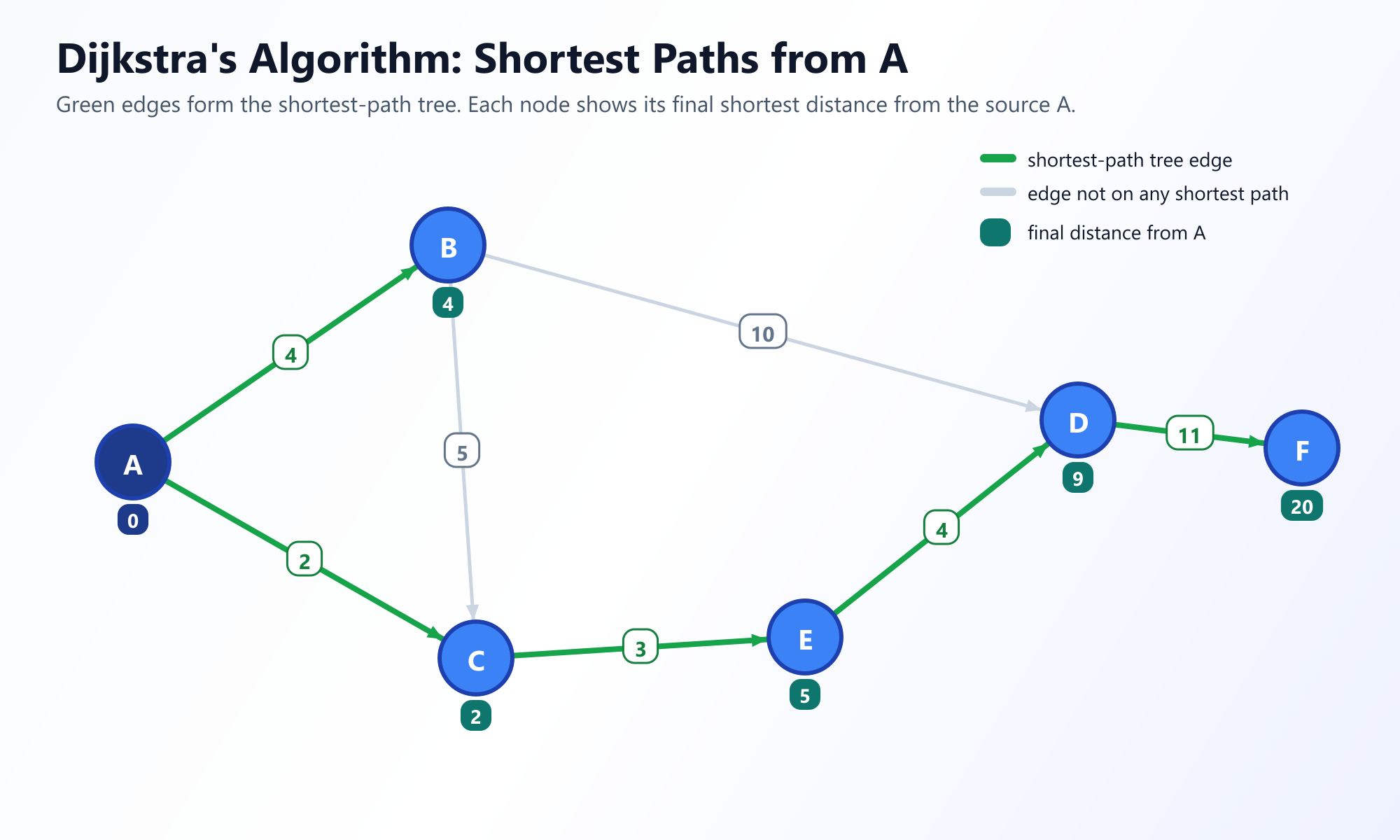
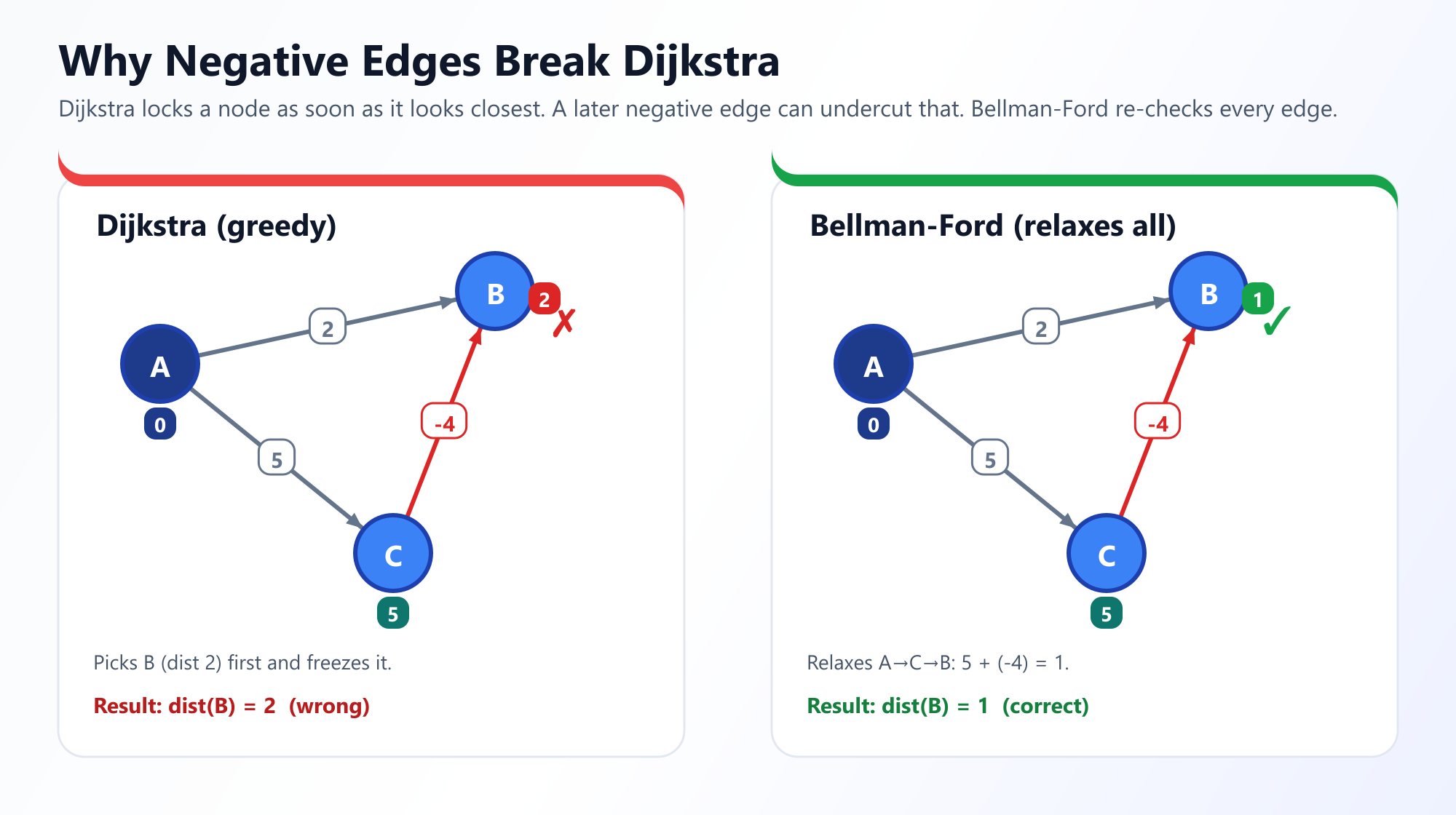
The Fatal Flaw: Negative Weights
Dijkstra's greedy nature makes it incredibly fast, running in O((V + E) log V) time. However, this greed comes with a fatal flaw: It assumes that adding an edge to a path can never make the path shorter. Therefore, if a graph contains negative edge weights (representing a profit, or time-travel, or energy regeneration), Dijkstra will fail silently and return incorrect results.
3. Bellman-Ford Algorithm: Handling the Negative
When you cannot guarantee that all edge weights are positive, the Bellman-Ford algorithm steps in. While Dijkstra is a greedy algorithm, Bellman-Ford uses a Dynamic Programming approach. It is slower, but far more robust.
Instead of cleverly picking the closest node, Bellman-Ford takes a sledgehammer approach: It simply "relaxes" (updates the distances of) every single edge in the graph. And it does this V - 1 times (where V is the total number of vertices). Because the longest possible path without a cycle in a graph can only be V - 1 edges long, repeating the process this many times guarantees that the absolute shortest paths have rippled outward to every node.
Detecting Negative Cycles
Bellman-Ford's greatest superpower is its ability to detect Negative Weight Cycles. If a graph has a loop where the total sum of weights is negative, you could infinitely loop through that cycle to achieve a distance of negative infinity. Shortest paths are mathematically undefined in such graphs. Bellman-Ford detects this by running the edge-relaxation process one final time (the V-th time). If any distance is still capable of being reduced, a negative cycle exists.
Implementation in Python
def bellman_ford(graph, num_vertices, start):
    distances = {vertex: float('infinity') for vertex in range(num_vertices)}
    distances[start] = 0

    # Relax all edges V - 1 times
    for _ in range(num_vertices - 1):
        for u, v, weight in graph:
            if distances[u] != float('infinity') and distances[u] + weight < distances[v]:
                distances[v] = distances[u] + weight

    # Check for negative-weight cycles
    for u, v, weight in graph:
        if distances[u] != float('infinity') and distances[u] + weight < distances[v]:
            print("Graph contains a negative weight cycle!")
            return None

    return distances

# Graph represented as an Edge List: (source, destination, weight)
edges = [
    (0, 1, -1), (0, 2, 4), (1, 2, 3), (1, 3, 2), (1, 4, 2), (3, 2, 5), (3, 1, 1), (4, 3, -3)
]
print(bellman_ford(edges, 5, 0))
The time complexity is a hefty O(V * E), making it unsuitable for massive networks like social media graphs, but perfect for specialized systems like financial currency arbitrage detection.
4. Floyd-Warshall Algorithm: The All-Pairs Solution
Both Dijkstra and Bellman-Ford are Single-Source shortest path algorithms. They calculate the distance from one specific starting node to all other nodes. But what if you are designing a routing table or a flight matrix, and you need to know the shortest path from every node to every other node simultaneously?
You could run Dijkstra V times, but the Floyd-Warshall Algorithm provides an incredibly elegant, pure Dynamic Programming alternative. It computes the shortest path between all pairs of vertices in a single, compact block of logic.
The Mechanics
Floyd-Warshall uses a 2D adjacency matrix. It iterates through every possible intermediate vertex k. For every pair of vertices (i, j), it asks a simple question: "Is it shorter to go directly from i to j, or is it shorter to go from i to k, and then from k to j?"
![The core Floyd-Warshall relaxation step. A triangle of nodes i, j and k. The direct edge i to j has weight 8, while the path i to k to j costs 3 plus 2 equals 5. Because 5 is smaller, dist[i][j] is updated from 8 to 5.](/articles/img/floyd-warshall-relaxation.png)
Implementation in Python
def floyd_warshall(graph, V):
    # Initialize the distance matrix
    dist = [[float('infinity') for _ in range(V)] for _ in range(V)]

    # Set the diagonal to 0, and initialize given edges
    for i in range(V):
        dist[i][i] = 0
    for u, v, w in graph:
        dist[u][v] = w

    # Core logic: check every intermediate vertex k
    for k in range(V):
        for i in range(V):
            for j in range(V):
                # Update distance if path through k is shorter
                dist[i][j] = min(dist[i][j], dist[i][k] + dist[k][j])

    return dist
The beauty of Floyd-Warshall lies in its simplicity, consisting of just three tightly nested loops. However, this results in a rigid time complexity of O(V³). It is exclusively used for dense graphs or graphs with a relatively small number of vertices.
5. Comprehensive Comparison
| Algorithm | Time Complexity | Handles Negative Weights? | Best Use Case |
|---|---|---|---|
| Dijkstra | O((V + E) log V) |
No (Fails silently) | GPS navigation, standard network routing, massive sparse graphs. |
| Bellman-Ford | O(V * E) |
Yes (And detects cycles) | Financial arbitrage, systems with penalties/costs. |
| Floyd-Warshall | O(V³) |
Yes | Flight network matrices, dense graphs, computing all pairs. |
Frequently Asked Questions
How do Dijkstra's and Bellman-Ford algorithms differ?
Dijkstra's is a greedy algorithm that runs in O((V + E) log V) but fails on negative weights. Bellman-Ford runs in O(VE), but can handle negative weights and detect negative cycles.
What is the Floyd-Warshall algorithm used for?
It is an all-pairs shortest path algorithm using dynamic programming, finding the shortest paths between all pairs of nodes in O(V³) time.
How does the A* algorithm optimize shortest path searches?
A* optimizes the search by using heuristics to estimate distance to the goal, focusing the search direction towards the target rather than exploring blindly in all directions.