
Table of Contents
- 1. What is the A* search algorithm?
- 2. Where A* came from: Hart, Nilsson and Raphael (1968)
- 3. The evaluation function f(n) = g(n) + h(n)
- 4. How A* runs, step by step
- 5. A worked example on a weighted graph
- 6. Admissible and consistent heuristics
- 7. Why A* is optimal, and when it is not
- 8. Time and space complexity
- 9. How to design a good heuristic
- 10. A* vs Dijkstra, UCS, greedy best first and BFS
- 11. Variants of A* worth knowing
- 12. Common mistakes in A* implementations
- 13. Where A* is actually used
- 14. Frequently asked questions
1. What is the A* search algorithm?
A* (pronounced "A star") is a best first graph search algorithm that finds a minimum cost path from a start node to a goal node. In artificial intelligence it is classified as an informed search: unlike breadth first search or uniform cost search, which only know what has already been paid, A* also uses an estimate of what still lies ahead.
Every node A* keeps on its frontier carries three numbers:
- g(n): the exact cost of the best path found so far from the start node to
n. - h(n): the heuristic, an estimate of the cheapest cost from
nto a goal. - f(n) = g(n) + h(n): the estimated cost of the cheapest complete solution that passes through
n.
The algorithm repeatedly expands the frontier node with the smallest f. That single rule produces the property A* is famous for: if the heuristic never overestimates the real remaining cost, the first goal node A* removes from the frontier lies on an optimal path.
Nothing in that definition mentions grids or video games. A* is defined on any weighted graph with non negative edge costs. The graph can be a road network, a tile map, the state space of a sliding tile puzzle, a robot's configuration space, or the set of partial plans inside an automated planner. Grid pathfinding is simply the picture that is easiest to draw, and it is covered in the companion guide on A* pathfinding on grids.
2. Where A* came from: Hart, Nilsson and Raphael (1968)
Peter E. Hart, Nils J. Nilsson and Bertram Raphael, working at the Stanford Research Institute, published "A Formal Basis for the Heuristic Determination of Minimum Cost Paths" in IEEE Transactions on Systems Science and Cybernetics, volume 4, issue 2, pages 100 to 107, July 1968. The practical motivation was Shakey, the SRI mobile robot, which had to plan its own route through a suite of rooms rather than follow a scripted track.
Two contributions from that paper still define the subject:
- It separated the search procedure from the knowledge inside it. The same loop becomes a different algorithm depending on which
hyou hand it. Search strategy became a parameter rather than a design decision. - It proved the guarantees. If
hnever overestimates the true remaining cost, the procedure returns a minimum cost path. A companion result showed that no other algorithm with access to the same heuristic information can expand fewer nodes and still guarantee optimality.
The name is a piece of notation that stuck. The 1968 paper marks optimal quantities with a star: g* is the least cost from the start to a node, h* the least cost from that node on to a goal, and f* their sum. The bare procedure is called A, and A* is the version of it that attains those quantities, the one whose heuristic never overestimates h*. It is not an abbreviation and it does not stand for anything.
A 1972 note in the SIGART Newsletter corrected the original optimality argument. The 1968 proof leaned on what the authors called the consistency assumption, and the correction made explicit what has to change when a heuristic is admissible but not consistent: already expanded nodes must be allowed to be reopened. That distinction is section 6 below, and it is still the single most common source of silently wrong A* implementations more than fifty years later.
If a citation is what brought you here: Hart, P. E., Nilsson, N. J., and Raphael, B. (1968). "A Formal Basis for the Heuristic Determination of Minimum Cost Paths." IEEE Transactions on Systems Science and Cybernetics 4(2), 100 to 107.
3. The evaluation function f(n) = g(n) + h(n)
Everything A* does follows from how it ranks its frontier. The evaluation function splits the estimate of a solution into a part that is known exactly and a part that is guessed:
f(n) = g(n) + h(n)

g(n)   cost already paid     exact, measured along the path actually taken
h(n)   cost still to pay     estimated by the heuristic function
f(n)   total estimate        the value the priority queue sorts on
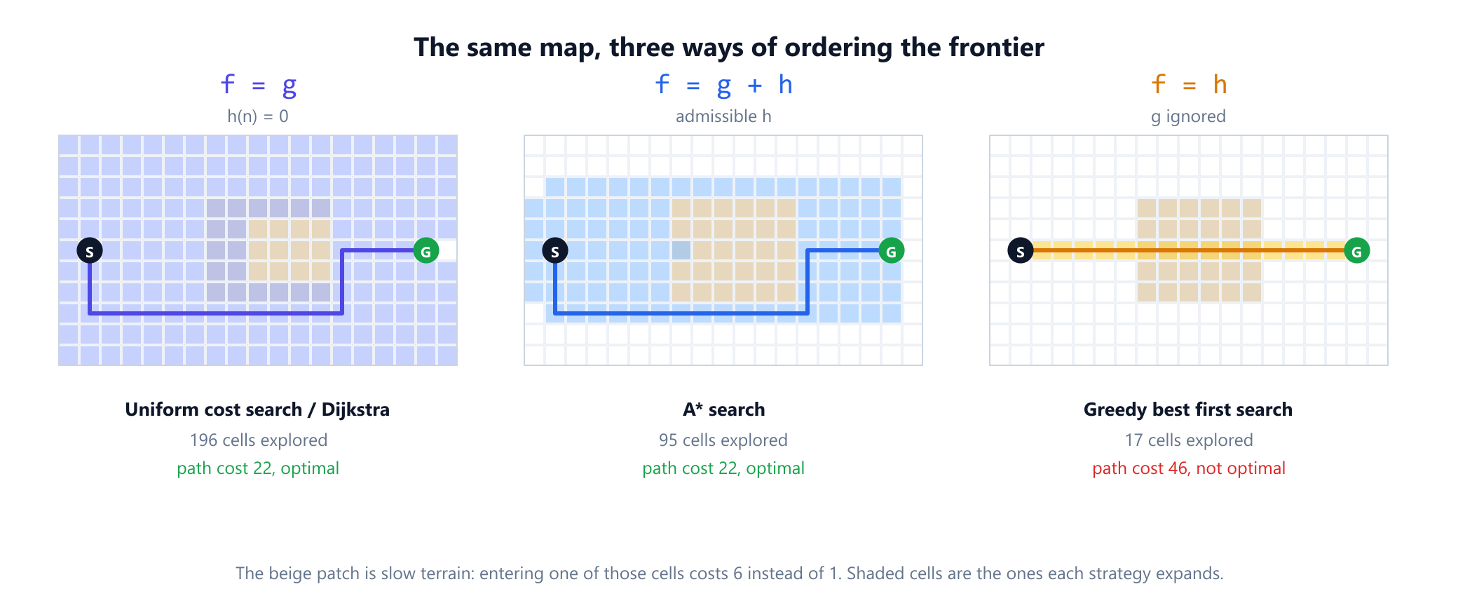
The value of that design is that one component controls the entire behaviour of the search:
- h(n) = 0 everywhere. Then
f = gand A* degenerates into uniform cost search, which on a graph with non negative weights is exactly Dijkstra's algorithm. Correct, but uninformed: it expands every node cheaper than the goal, in every direction. - h(n) = h*(n), the true remaining cost. A* walks straight down an optimal path and expands almost nothing else. This is the theoretical ceiling, and it is unavailable in practice because computing
h*is the very problem you were trying to solve. - Ignore g and rank on h alone. That is greedy best first search. It is fast, it is often badly wrong, and it carries no optimality guarantee.
- Reweight: f = g + w × h with w > 1. Weighted A* trades a bounded amount of solution quality for a large amount of speed. The path it returns is never worse than
wtimes the optimal cost.
Read that list as a scale of how much you trust the estimate. A* sits in the middle and spends effort in proportion to how little the heuristic knows: a sharp heuristic produces a search that looks like a straight line, a weak one produces a search that looks like Dijkstra.
4. How A* runs, step by step
The frontier is a priority queue, traditionally called OPEN, ordered by f. A map of best known g values and a map of parent pointers complete the state.
function a_star(start, goal, h):
    open   = priority queue ordered by f        # the frontier
    g      = map with default infinity          # best known cost from start
    parent = map                                # for path reconstruction

    g[start] = 0
    open.push(start, h(start))

    while open is not empty:
        current = open.pop_min()                # node with the smallest f
        if current == goal:
            return reconstruct(parent, goal)    # goal test on pop, not on generate

        for (next, cost) in edges(current):
            tentative = g[current] + cost
            if tentative < g[next]:             # a cheaper route to next
                g[next]      = tentative
                parent[next] = current
                open.push_or_update(next, tentative + h(next))

    return failure                              # the goal is unreachable
Four implementation details carry most of the subtlety:
- The goal test happens when a node is popped, not when it is generated. A goal can be generated early along an expensive route. Returning at that moment gives you a path, just not the cheapest one. The worked example below contains a case where testing on generation costs 7 units out of 13.
- Relaxation is guarded by
tentative < g[next], not by membership of a closed set. Written this way, the loop reopens an already expanded node automatically when a cheaper route to it turns up later, which is what makes it correct for any admissible heuristic. - Most priority queues have no decrease key operation. Production code usually pushes a duplicate entry with the better
fand discards stale entries as they come out. This is called lazy deletion: it costs a little memory and saves a lot of bookkeeping. - The path is recovered backwards. Follow parent pointers from the goal to the start and reverse the list. A* never stores paths, only one parent per node.
5. A worked example on a weighted graph
Grid animations hide the arithmetic. Here is a small weighted graph, the kind used in AI courses, traced by hand from start to finish.
Six nodes: S (start), A, B, C, D and G (goal). Edge costs are road distances, and the heuristic h is a straight line distance to G, which is what makes it admissible: a straight line is never longer than a road.
Edges (undirected, cost)      Heuristic h(n)
S-A  4      A-C  5            S = 11    C = 5
S-B  3      A-D  12           A =  9    D = 3
S-G  20     B-D  7            B =  8    G = 0
C-G  6      D-G  3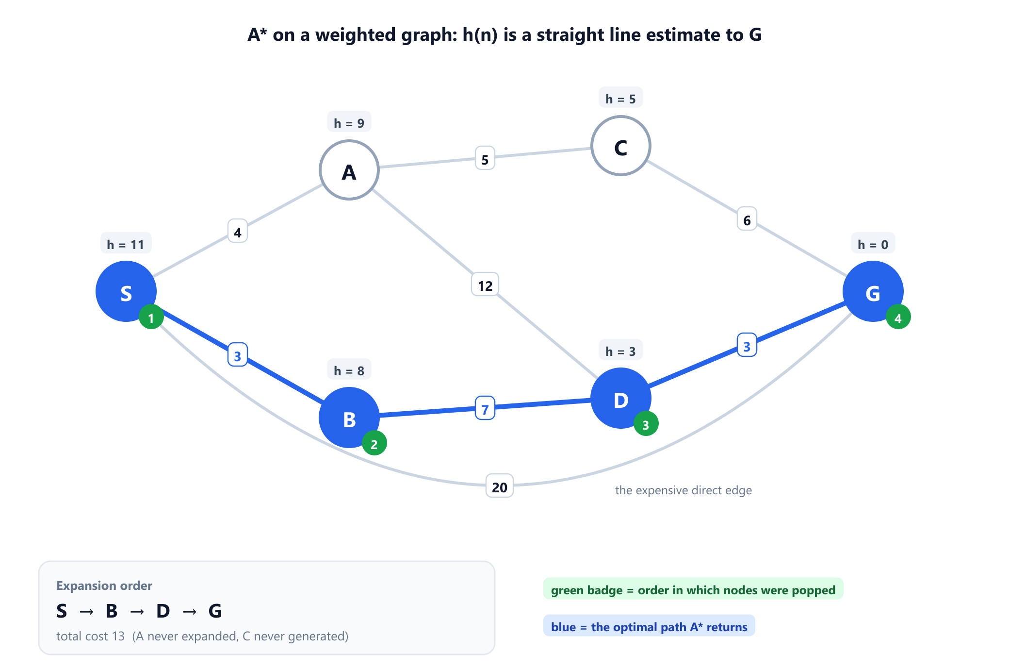
A* pops the node with the smallest f, breaking ties in favour of the smaller h, which is the standard tie break because it prefers nodes nearer the goal:
| Step | Popped | g | h | f | Frontier after the step |
|---|---|---|---|---|---|
| 1 | S | 0 | 11 | 11 | B 11, A 13, G 20 |
| 2 | B | 3 | 8 | 11 | A 13, D 13, G 20 |
| 3 | D | 10 | 3 | 13 | G 13 (improved from 20), A 13 |
| 4 | G | 13 | 0 | 13 | goal popped, search ends |
The answer is S → B → D → G at a cost of 13. Three things in that trace are worth pausing on:
- The goal was generated in step 1 with f = 20 and ignored. An implementation that returns as soon as it generates the goal would have reported a path costing 20, which is 54 percent worse than optimal. A* keeps it on the frontier and only accepts it once nothing cheaper remains.
- Node C was never even generated. Dijkstra on the same graph expands every node with distance below 13, which includes C at 9. A* never touches it because the frontier never gets that far.
- Node A was generated but never expanded. Its
fof 13 ties with the goal, and since a tie atf = C*can be resolved either way, A never became worth opening. That is exactly the boundary case the optimal efficiency theorem talks about.
6. Admissible and consistent heuristics
Two properties of h are worth distinguishing carefully, because they are often used as though they were the same thing and they are not.
Admissibility
A heuristic is admissible if it never overestimates:
h(n) <= h*(n)   for every node n
                where h*(n) is the true cheapest cost from n to a goal
Admissibility is optimism. The heuristic is allowed to be wildly wrong as long as it errs on the low side. h = 0 is admissible, which is why Dijkstra is a special case of A* rather than a rival to it.
Consistency, also called monotonicity
A heuristic is consistent if it satisfies a triangle inequality along every edge:
h(n) <= cost(n, n') + h(n')   for every edge n to n'
h(goal) = 0
In words: taking one step can never reduce your estimate by more than the step actually cost. Consistency is the stronger property. Every consistent heuristic is admissible; the reverse is false.
The practical consequence is precise. When h is consistent, f never decreases along a path, so the first time A* pops a node, its g value is already optimal. That is what licenses the familiar optimisation of putting expanded nodes into a closed set and never looking at them again.
When h is only admissible, that licence is withdrawn. A cheaper route to an already expanded node can still be discovered, and if the implementation refuses to reopen it, the final answer can be wrong. Here is a graph where exactly that happens:
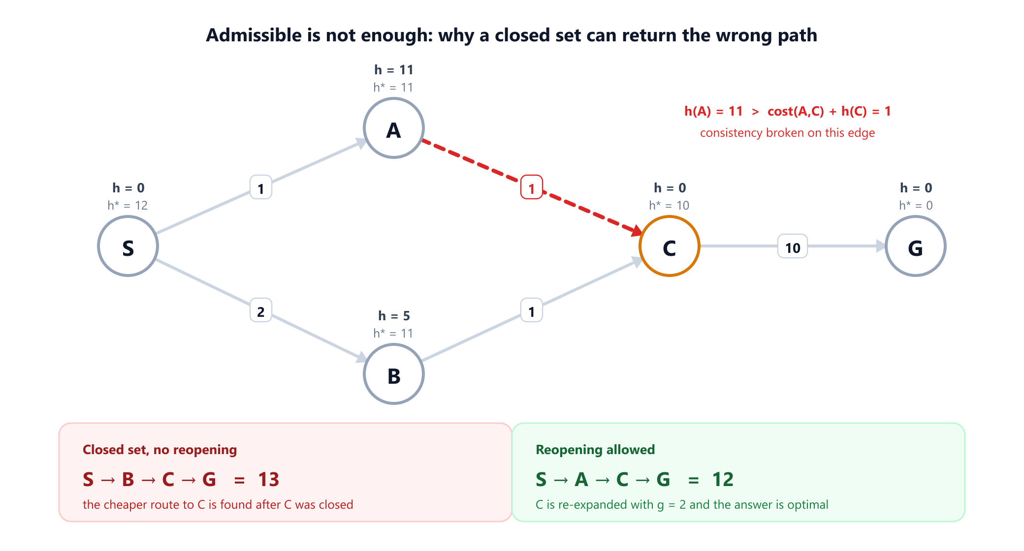
Edges (directed, cost)     Heuristic h(n)     True cost h*(n)
S -> A   1                 S =  0             S = 12
S -> B   2                 A = 11             A = 11
A -> C   1                 B =  5             B = 11
B -> C   1                 C =  0             C = 10
C -> G  10                 G =  0             G =  0

Every h(n) <= h*(n), so the heuristic is admissible.
Edge A -> C breaks consistency: h(A) = 11 > cost(A,C) + h(C) = 1.
Trace it: A* pops S (f = 0), generating A at f = 1 + 11 = 12 and B at f = 2 + 5 = 7. It pops B (f = 7) and generates C with g = 3, f = 3. It pops C (f = 3), closes it with g = 3, and generates G at f = 13. Only then does it pop A (f = 12) and discover a route to C costing just 2. If C is closed and closed means final, that discovery is thrown away and the algorithm returns 13 instead of the optimal 12.
Two ways out, and you should pick one deliberately: prove your heuristic is consistent and keep the closed set optimisation, or write the relaxation as tentative < g[next] with no closed set check so reopening happens on its own. The reassuring news is that nearly every heuristic used in practice, including straight line distance, Manhattan distance on a uniform cost grid, and any heuristic derived from a relaxed problem, is consistent. That is precisely why this bug can survive years of use before a strange map exposes it.
7. Why A* is optimal, and when it is not
The optimality argument is short enough to hold in your head, and worth knowing because it tells you exactly which assumption to check when A* misbehaves.
Let C* be the cost of an optimal solution. Suppose A* is about to pop a goal node G2 reached along a suboptimal path, so g(G2) > C*. Since h(G2) = 0, its priority is f(G2) = g(G2) > C*. Now consider any optimal path from the start to a real optimal goal. At the moment before the pop, that path must have at least one node n sitting on the frontier, because the start was expanded and the goal was not. For that node, g(n) is the optimal cost to reach it and, because h is admissible, f(n) = g(n) + h(n) <= g(n) + h*(n) = C*. So f(n) <= C* < f(G2), and A* would have popped n first. The contradiction proves that the first goal popped is optimal.
The same reasoning gives you the conditions under which the guarantee fails:
- The heuristic overestimates somewhere. The inequality
f(n) <= C*breaks, and A* can walk past the optimal path. This is not always a disaster, but the guarantee is gone and you should say so in the code. - Negative edge costs. A* assumes costs are non negative, as does Dijkstra. With negative edges the frontier ordering means nothing. Use Bellman Ford instead.
- Costs that change during the search. Static A* has no answer for a door that closes mid plan. That is what D* Lite and lifelong planning A* exist for.
- Infinite or unbounded graphs. Completeness needs a finite branching factor and edge costs bounded below by some positive epsilon. Without that, A* can chase an infinite sequence of ever cheaper steps and never terminate.
One further result rounds out the theory. Dechter and Pearl proved in 1985 that A* is optimally efficient: no other optimal algorithm using the same heuristic information is guaranteed to expand fewer nodes. Every node with f(n) < C* must be expanded by any such algorithm, and A* expands exactly those, plus some subset of the nodes sitting exactly at f(n) = C*. There is no cleverer scheduling to be found; the only remaining lever is a better heuristic.
8. Time and space complexity
The textbook figure is O(bd), where b is the branching factor and d is the depth of the optimal solution, and that number is honest but not very informative. The sharper statement is about the heuristic's error. The number of nodes A* expands grows exponentially unless the error of the heuristic is bounded logarithmically in the true cost:
|h(n) - h*(n)| <= O(log h*(n))Almost no heuristic used in practice meets that bar, so the honest reading is that A* is exponential in the worst case and that a good heuristic reduces the base of the exponent rather than removing it. On an explicit graph that you already hold in memory, the accounting is the same as Dijkstra's: O(E log V) with a binary heap, since every edge triggers at most one queue update. The interesting question is not the bound but how few of those V and E the search ever touches.
Memory is the constraint that actually bites. A* keeps every generated node in memory, both the frontier and the explored set, so its space complexity matches its time complexity. Real systems run out of RAM long before they run out of patience. This single fact explains the entire family of variants in section 11: iterative deepening A*, simplified memory bounded A*, and beam style truncations all exist to trade optimality or repeated work for a frontier that fits.
9. How to design a good heuristic
Since the algorithm is fixed and provably efficient, all of the engineering lives in h. There is a reliable recipe for producing one.
Relax the problem
Take the real problem, delete a constraint, and solve what is left exactly. The exact cost of a relaxed problem is always a lower bound on the real cost, so it is admissible by construction, and because a relaxed solution can be built one step at a time it is consistent as well.
The 8 puzzle is the standard illustration. A tile may move to the adjacent blank square. Delete constraints and two classic heuristics fall out:
- h1, misplaced tiles. Allow any tile to teleport anywhere in one move. Then the cost is simply the number of tiles not in their goal position.
- h2, Manhattan distance. Allow a tile to move to any adjacent square, blank or not. Then the cost is the sum, over all tiles, of the horizontal plus vertical distance to that tile's goal square.
Both are admissible. The difference in practice is dramatic: on random 8 puzzle instances requiring 12 moves, the classic comparison reported by Russell and Norvig has iterative deepening search generating on the order of 3.6 million nodes, A* with h1 generating a few hundred, and A* with h2 generating fewer than a hundred. At depth 24 the gap widens to roughly 39,000 nodes for h1 against roughly 1,600 for h2. Same algorithm, same code, different h.
Prefer a dominant heuristic
If h2(n) >= h1(n) for every node and both are admissible, then h2 dominates h1 and A* with h2 never expands more nodes. Bigger is better, right up to the ceiling of h*. This is why Manhattan distance beats misplaced tiles: it is always at least as large and never overestimates.
Combine several heuristics
If you have several admissible heuristics and none dominates the others, take their maximum. The maximum of admissible heuristics is admissible, and it dominates all of them. The cost is that you now evaluate several functions per node, so the win has to be paid for in evaluation time.
Precompute with pattern databases
For a fixed goal state, solve subproblems exhaustively in advance and store the exact costs in a table. A pattern database for a subset of the puzzle tiles gives a far stronger admissible bound than any formula. This is the same idea that makes landmark based routing work on continental road networks: precompute exact distances to a handful of landmarks, then use the triangle inequality to bound the rest.
On grids, choose the metric that matches the moves
Manhattan distance for 4 directional movement, Euclidean for any angle movement, Chebyshev or octile for 8 directional grids. Choosing a metric that allows less freedom than the movement rules do makes the heuristic inadmissible and quietly destroys the optimality guarantee. The grid pathfinding guide works through all three with worked numbers.
10. A* vs Dijkstra, UCS, greedy best first and BFS
Every one of these is the same loop with a different priority. That is the most useful way to remember them.
| Algorithm | Frontier priority | Optimal? | Use it when |
|---|---|---|---|
| Breadth first search | insertion order (FIFO) | Yes, if all edges cost the same | Unweighted graphs, fewest hops |
| Uniform cost search / Dijkstra | f = g | Yes | Weighted graph, no useful estimate available, or many goals at once |
| Greedy best first search | f = h | No | You need any solution fast and quality is negotiable |
| A* | f = g + h | Yes, if h is admissible | Single goal, a decent estimate exists, the path must be shortest |
| Weighted A* | f = g + w × h | Within a factor of w | A* is too slow and a bounded detour is acceptable |
The intuition behind the A* against Dijkstra comparison is geometric. Dijkstra expands everything with g(n) < C*, which on an open map is a circle around the start. A* expands everything with g(n) + h(n) < C*, which is an ellipse with the start and the goal as its focal points. The sharper the heuristic, the flatter that ellipse becomes, until it collapses onto the path itself. Both return the same optimal answer; they differ only in how much of the map they had to look at to be sure. For a broader map of the family, see the overview of shortest path algorithms, and for the traversal foundations underneath all of it, BFS vs DFS.
11. Variants of A* worth knowing
Nearly every named variant is a response to one of two pressures: memory, or the need to answer before the optimum is proved.
- Weighted A* multiplies the heuristic by
w > 1. Solutions are guaranteed within a factorwof optimal, and in practice are usually far better than that bound while running an order of magnitude faster. - IDA* (iterative deepening A*) runs repeated depth first searches with an increasing
fcutoff. Memory drops to the depth of the search, and the price is re-expanding nodes on every iteration. This is the standard tool for puzzles with enormous state spaces. - SMA* (simplified memory bounded A*) uses all the memory you give it and, when it runs out, drops the worst leaf while remembering its value in the parent. It remains optimal if the optimal path fits in memory.
- ARA* and other anytime variants start with a large
w, return a solution quickly, then keep improving it while time remains, tightening the bound as they go. - D* and D* Lite repair an existing plan when edge costs change, instead of replanning from scratch. This is what a robot discovering an unmapped obstacle needs.
- Jump point search exploits the symmetry of uniform cost grids to skip whole runs of identical cells. Same answer as A*, often an order of magnitude fewer expansions, grids only.
- Bidirectional A* searches forward from the start and backward from the goal at once. It is powerful and subtle, since the stopping condition and the heuristic consistency requirements both become harder.
- ALT and contraction hierarchies are what production route planners actually run. Plain A* is too slow on continental road networks, so these precompute landmark distances or shortcut edges and then search a much smaller effective graph.
12. Common mistakes in A* implementations
Most A* bugs do not crash. They return a path that is slightly too long, on some inputs, sometimes. These are the recurring causes:
- Mismatched units.
gmeasured in seconds andhmeasured in metres is the classic. Ifhis even slightly overscaled it stops being admissible and the guarantee is gone. Convert both to the same currency before adding them. - A closed set with an inconsistent heuristic. The failure mode from section 6. If you cannot prove consistency, allow reopening.
- No tie breaking. When many nodes share the same
f, an arbitrary order makes A* explore a wide plateau of equally promising cells. Breaking ties towards the smallerhcosts nothing and keeps every guarantee intact. The other common trick, scalinghby 1 + epsilon, narrows the search dramatically on grids but makes the heuristic very slightly inadmissible, so use it knowing you have traded the proof for the speed. - Testing the goal on generation. Fast, tempting, and it silently returns suboptimal paths, as the worked example showed.
- Floating point comparison. Euclidean heuristics produce irrational values, and strict equality checks on
fbehave unpredictably. Compare with a tolerance, or keep costs in integers. - Forgetting h(goal) = 0. A non zero estimate at the goal breaks consistency at the last edge and can distort the whole search.
- Recomputing h on every queue operation. The heuristic is called constantly. Cache it on the node; profilers find this one over and over.
- Mutable states used as dictionary keys. In puzzle search, a board mutated in place corrupts the visited set. Store an immutable encoding.
13. Where A* is actually used
A* earns its place anywhere a best sequence of decisions has to be found in a space too large to enumerate:
- Robotics and motion planning. The original Shakey application, still current: grid and lattice planners for mobile robots, warehouse fleets and autonomous vehicles, usually with D* Lite handling replanning as the world changes.
- Game AI. Units routing across navigation meshes and tile maps, typically with hierarchical decomposition on top so that a long path is planned coarsely first and refined locally.
- Route planning. Journey planners run A* derivatives with landmark heuristics or contraction hierarchies, which is how a continental route is returned in milliseconds.
- Puzzle and state space search. Sliding tile puzzles, Rubik's cube solvers and similar combinatorial problems, usually with IDA* and pattern databases because the state spaces are far too large for a frontier in memory.
- Automated planning. Classical planners search the space of world states with heuristics derived automatically from a relaxed version of the planning problem, which is the same relaxation recipe from section 9 applied mechanically.
- Bioinformatics. Multiple sequence alignment is a shortest path problem in a high dimensional lattice, and A* with an admissible bound is a standard exact method.
- Speech and language decoding. A* search over a word lattice, where
gis the score of the partial hypothesis andhbounds the best completion, remains a textbook decoding strategy.
The pattern is always the same. Model the problem as a graph, find an admissible lower bound on the remaining cost, and let the priority queue do the rest.
14. Frequently asked questions
Does A* always find the shortest path?
Yes, provided three conditions hold: the heuristic is admissible (it never overestimates the remaining cost), edge costs are non negative, and the implementation tests for the goal when a node is popped rather than when it is generated. If the heuristic is admissible but not consistent, the implementation must also allow already expanded nodes to be reopened. Break any one of those conditions and A* still returns a path, but it is no longer guaranteed to be the cheapest one.
What is the difference between A* and Dijkstra's algorithm?
They are the same algorithm with different priorities. Dijkstra orders its frontier by g(n), the cost already paid, so it expands outwards in every direction like a growing circle. A* orders by f(n) = g(n) + h(n), so the region it expands is an ellipse stretched from the start towards the goal. Setting h(n) = 0 turns A* into Dijkstra exactly. Dijkstra is the better choice when no useful estimate exists or when you need distances to many destinations at once; A* is the better choice for a single destination with a decent estimate available.
What is the difference between an admissible and a consistent heuristic?
Admissible means h(n) is never greater than the true remaining cost h*(n). Consistent, also called monotone, is the stronger triangle inequality h(n) <= cost(n, n') + h(n') for every edge, with h(goal) = 0. Every consistent heuristic is admissible, but not the reverse. Consistency matters because it guarantees that the first time A* pops a node, its g value is already optimal, which is what makes a closed set safe. With a merely admissible heuristic, a cheaper route to a closed node can still appear later and the node must be reopened.
What is the time and space complexity of A*?
In the worst case both are O(b^d), exponential in the depth of the solution. The number of expansions stays polynomial only when the heuristic error is bounded logarithmically, which almost never happens in practice, so a better heuristic reduces the base of the exponent rather than removing it. On an explicit graph already in memory, A* behaves like Dijkstra at O(E log V) with a binary heap. Space is the practical limit: A* stores every node it generates, which is why memory bounded variants such as IDA* and SMA* exist.
Why is it called A*, and is it an AI algorithm or a graph algorithm?
The star is the notation the 1968 paper uses for optimal quantities, as in g*, h* and f*: the bare procedure is called A, and A* is the version of it whose heuristic never overestimates, so it returns a least cost path. It is both an AI algorithm and a graph algorithm. It is taught in AI courses as the canonical informed search method, and it is a shortest path algorithm on weighted graphs. It is not machine learning: nothing is trained and no data is fitted. The knowledge lives entirely in the heuristic function you supply, although a learned model can perfectly well be used to supply one.
Is A* complete, and what happens if no path exists?
A* is complete on a graph with a finite branching factor whose edge costs are bounded below by some positive value: if a solution exists it will be found. When no path exists, the frontier empties after the entire reachable component has been expanded and the algorithm reports failure. That failure case is the expensive one, since proving that nothing exists means exploring everything reachable, which is a good reason to add a connectivity precheck on large maps.
See the frontier move
Run Dijkstra on your own graph in the interactive visualizer. It is A* with h set to zero, so what you watch flooding outwards is exactly the work a good heuristic removes.
Launch the visualizer