
Table of Contents
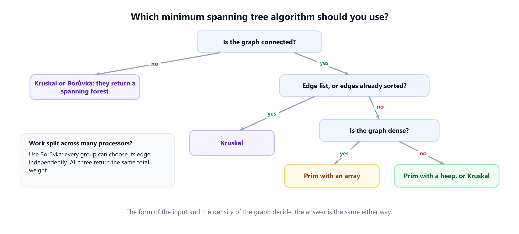
- 1. The short answer
- 2. One graph, three runs
- 3. Why all three are correct
- 4. When the trees differ
- 5. Speed: which one is faster, and when
- 6. The shape of your input
- 7. Disconnected graphs and stopping early
- 8. Negative weights, maximum trees and directed graphs
- 9. Prim is not Dijkstra
- 10. A tangled history
- 11. Where each one is used
- 12. Common mistakes
- 13. Glossary
- 14. Frequently asked questions
- 15. References
1. The short answer
Prim's algorithm, Kruskal's algorithm and Borůvka's algorithm all find a minimum spanning tree: the cheapest set of edges that connects every vertex of a weighted graph. They build it in different orders, and that decides which one suits a given graph. The guide to minimum spanning trees introduces the problem itself.
| Prim | Kruskal | Borůvka | |
|---|---|---|---|
| Strategy | Grow one tree outward from a start vertex | Take edges from cheapest up, skipping any that close a cycle | Every group picks its cheapest outgoing edge, all at once |
| Main data structure | Priority queue, or a plain array | Sorted edge list and union-find | Union-find, or relabelling |
| Time | O(E log V) with a binary heap, O(V2) with an array | O(E log E), nearly linear if the edges are already sorted | O(E log V) |
| Natural input | Adjacency list or matrix | Edge list | Edge list |
| Disconnected graph | Covers only the start vertex's component | Gives a spanning forest | Gives a spanning forest |
| Best for | Dense graphs, with the array version | Sparse graphs, presorted edges, clustering | Parallel and distributed computing |
Here V is the number of vertices and E the number of edges. In one sentence: use Kruskal when the graph is sparse or given as a list of edges, use Prim when it is dense or given as a matrix, and consider Borůvka when the work must be split across many processors. On a sparse graph Kruskal and Prim with a heap cost about the same, so the simpler code for your data is the right choice.
2. One graph, three runs
Eight villages, A to H, want to be joined by water pipes. There are 14 possible routes, each with a cost in kilometres of trench, and every village must end up connected to every other. Together, all 14 routes would cost 117.
A-B 3    A-C 6    B-C 4    B-D 13   C-D 7    C-E 12   D-E 2
D-F 11   E-F 8    E-G 14   E-H 5    F-G 1    F-H 15   G-H 16

8 villages, 14 possible pipes
A cheapest connection uses exactly 7 pipes, one fewer than the number of villages, because any extra pipe would close a loop that could be removed to save money. This graph has 712 spanning trees, and exactly one of them costs the minimum of 30. The program below implements all three algorithms and runs them on it.
import heapq

PIPES = [('A', 'B', 3), ('A', 'C', 6), ('B', 'C', 4), ('B', 'D', 13), ('C', 'D', 7),
         ('C', 'E', 12), ('D', 'E', 2), ('D', 'F', 11), ('E', 'F', 8), ('E', 'G', 14),
         ('E', 'H', 5), ('F', 'G', 1), ('F', 'H', 15), ('G', 'H', 16)]

class Groups:
    """Union-find: which group is each vertex in?"""
    def __init__(self, items):
        self.parent = {x: x for x in items}
    def find(self, x):
        while self.parent[x] != x:
            self.parent[x] = self.parent[self.parent[x]]   # path halving
            x = self.parent[x]
        return x
    def union(self, a, b):
        ra, rb = self.find(a), self.find(b)
        if ra == rb:
            return False
        self.parent[ra] = rb
        return True

def vertices(edges):
    return sorted({x for u, v, _ in edges for x in (u, v)})

def prim(edges, start):
    """Grow one tree: always add the cheapest edge that leaves it."""
    adj = {v: [] for v in vertices(edges)}
    for u, v, w in edges:
        adj[u].append((w, u, v))
        adj[v].append((w, v, u))
    seen, heap, tree = {start}, list(adj[start]), []
    heapq.heapify(heap)
    while heap:
        w, u, v = heapq.heappop(heap)
        if v in seen:
            continue                                  # both ends are already in the tree
        seen.add(v)
        tree.append((u, v, w))
        for e in adj[v]:
            if e[2] not in seen:
                heapq.heappush(heap, e)
    return tree

def kruskal(edges):
    """Take the edges from cheapest up, skipping any that would close a cycle."""
    groups, tree = Groups(vertices(edges)), []
    for u, v, w in sorted(edges, key=lambda e: e[2]):
        if groups.union(u, v):
            tree.append((u, v, w))
    return tree

def boruvka(edges):
    """In each round, every group picks its cheapest outgoing edge at the same time."""
    groups, tree, rounds = Groups(vertices(edges)), [], []
    while True:
        cheapest = {}
        for u, v, w in edges:
            ru, rv = groups.find(u), groups.find(v)
            if ru != rv:
                for r in (ru, rv):                    # ties broken the same way everywhere
                    if r not in cheapest or (w, u, v) < cheapest[r]:
                        cheapest[r] = (w, u, v)
        if not cheapest:
            return tree, rounds
        added = []
        for w, u, v in sorted(set(cheapest.values())):
            if groups.union(u, v):
                added.append((u, v, w))
        tree += added
        rounds.append(added)

def show(tree):
    return ' '.join(f'{u}{v}:{w}' for u, v, w in tree) + f'   total {sum(w for *_, w in tree)}'

print('Prim    ', show(prim(PIPES, 'A')))
# Prim     AB:3 BC:4 CD:7 DE:2 EH:5 EF:8 FG:1   total 30
print('Kruskal ', show(kruskal(PIPES)))
# Kruskal  FG:1 DE:2 AB:3 BC:4 EH:5 CD:7 EF:8   total 30
tree, rounds = boruvka(PIPES)
print('Boruvka ', show(tree))
# Boruvka  FG:1 DE:2 AB:3 BC:4 EH:5 CD:7 EF:8   total 30
for i, added in enumerate(rounds, 1):
    print('round', i, show(added))
# round 1 FG:1 DE:2 AB:3 BC:4 EH:5   total 15
# round 2 CD:7 EF:8   total 15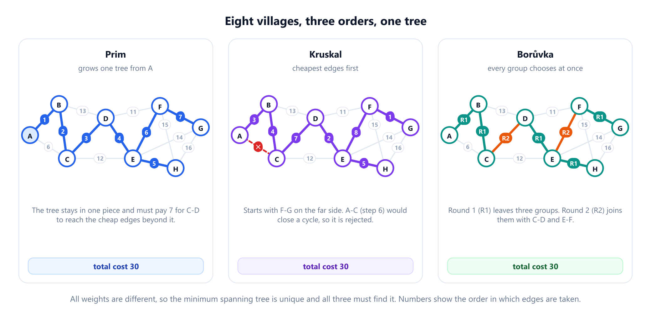
The three orders tell the story of each method:
- Prim starts at
Aand always extends the one tree it has. It takesA-Bat 3,B-Cat 4 and then has to pay 7 forC-Dbefore it can reach the cheap edgesD-EandF-Gfurther on. - Kruskal ignores geography. It takes
F-Gat 1 first, on the far side of the graph, and works up the price list. When it reachesA-Cat 6,AandCare already joined throughB, so it rejects that pipe. AfterE-Fat 8 it has 7 pipes and can stop, without ever looking at the six most expensive routes. - Borůvka works in rounds. In round 1 every village picks its cheapest pipe, which gives five different pipes and three groups:
{A, B, C},{D, E, H}and{F, G}. In round 2 each group picks its cheapest pipe to another group, andC-DandE-Ffinish the job.
3. Why all three are correct
Different as they look, all three rest on the same fact about cuts. A cut divides the vertices into two groups, as the guide to the minimum cut explains. The cut property says: for any cut, the cheapest edge crossing it belongs to a minimum spanning tree, and when weights are all different it belongs to every one. The proof is an exchange. Take a spanning tree that does not use that edge and add it: this closes a cycle, the cycle must cross the cut a second time on some dearer edge, and removing that dearer edge gives a cheaper tree.
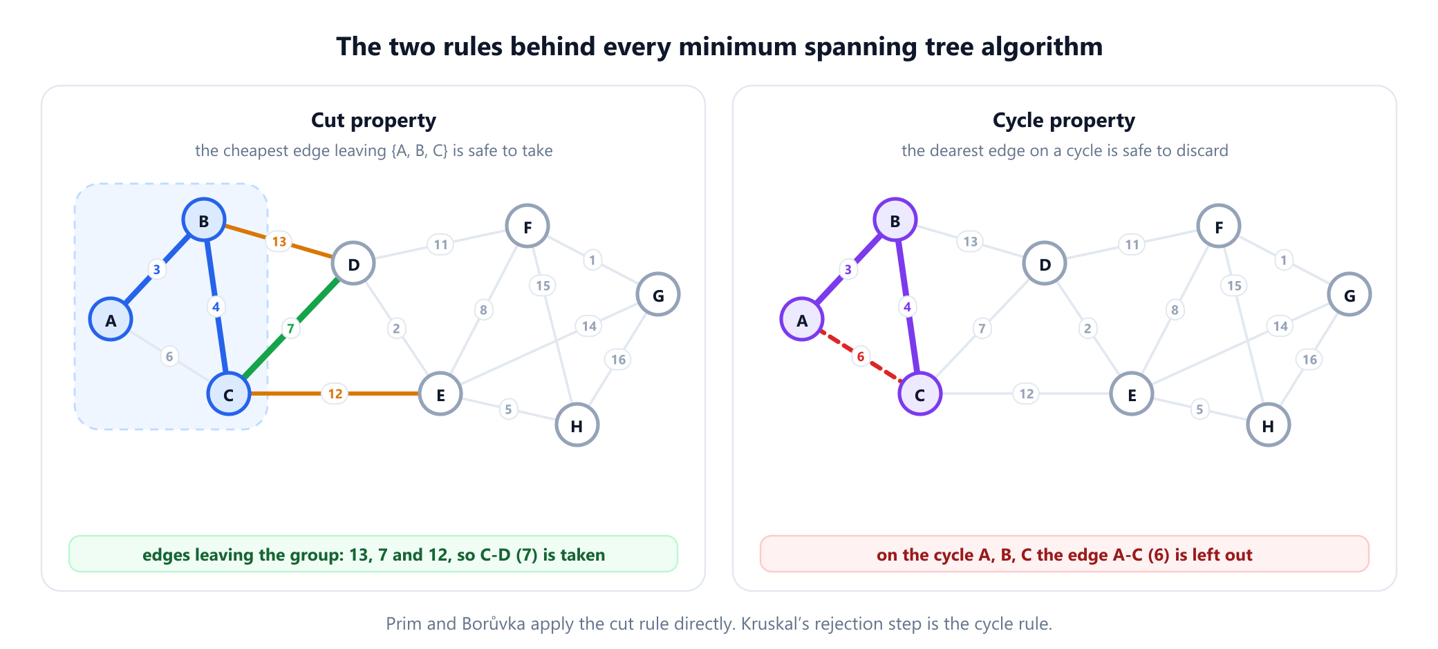
Each algorithm applies this rule to a different cut:
- Prim uses the cut between its tree and everything else. In the picture, the tree
{A, B, C}can leave along three edges, and the cheapest,C-Dat 7, is added. - Kruskal uses the cut around one of the two groups the edge joins. Edges are taken in increasing order, so when an edge joins two groups, nothing cheaper leaves either of them.
- Borůvka uses the cut around each group, for every group at the same time.
The mirror image is the cycle property: the most expensive edge on any cycle can be left out of a minimum spanning tree. That is Kruskal's rejection step. When A-C at 6 would close the cycle A, B, C, it is the dearest edge on that cycle, because every other edge on it was taken earlier. A minimum spanning tree never needs that edge.
4. When the trees differ
If all edge weights are different, the minimum spanning tree is unique, so all three algorithms must return exactly the same edges, as they do on the example. With equal weights there may be several minimum spanning trees, all with the same total, and which one you get depends on the algorithm and even on the order of the input. Change A-C to cost 4, the same as B-C, and there are exactly two minimum spanning trees:
PIPES = [('A', 'B', 3), ('A', 'C', 6), ('B', 'C', 4), ('B', 'D', 13), ('C', 'D', 7),
         ('C', 'E', 12), ('D', 'E', 2), ('D', 'F', 11), ('E', 'F', 8), ('E', 'G', 14),
         ('E', 'H', 5), ('F', 'G', 1), ('F', 'H', 15), ('G', 'H', 16)]

def kruskal(edges):
    parent = {x: x for u, v, _ in edges for x in (u, v)}
    def find(x):
        while parent[x] != x:
            x = parent[x]
        return x
    tree = []
    for u, v, w in sorted(edges, key=lambda e: e[2]):  # stable: ties keep their input order
        if find(u) != find(v):
            parent[find(u)] = find(v)
            tree.append(u + v)
    return sorted(tree), sum(w for u, v, w in edges if u + v in tree)

tied = [(u, v, 4 if (u, v) == ('A', 'C') else w) for u, v, w in PIPES]   # A-C now costs 4, like B-C
print(kruskal(tied))
# (['AB', 'AC', 'CD', 'DE', 'EF', 'EH', 'FG'], 30)
print(kruskal(tied[::-1]))
# (['AB', 'BC', 'CD', 'DE', 'EF', 'EH', 'FG'], 30)
Both trees cost 30 and differ in one pipe. Python's sort is stable, so equal edges keep their input order, and reversing the list changes which of the two is taken first. If your tests compare the exact edges of a tree, they can fail on a correct program; compare the total weight instead.
Ties are also the classic bug in Borůvka's algorithm. When two groups each choose between edges of equal weight, inconsistent choices can create a cycle. The program above avoids this by comparing (w, u, v) everywhere, so every group breaks ties the same way.
5. Speed: which one is faster, and when
| Version | Time | Where the time goes |
|---|---|---|
| Prim, binary heap | O(E log V) | Up to one heap operation per edge |
| Prim, plain array | O(V2) | Scanning all remaining vertices, once per vertex added |
| Prim, Fibonacci heap | O(E + V log V) | Fast theoretically, heavy constants in practice |
| Kruskal | O(E log E) | Sorting; the union-find work after that is almost linear |
| Borůvka | O(E log V) | At most log2 V rounds, each scanning every edge |
Since E is at most V2, log E is at most 2 log V, so O(E log E) and O(E log V) are the same class. The formulas alone do not separate the methods, so the program below counts basic steps, meaning comparisons, edge inspections and union-find hops, on two random graphs with 1,000 vertices. One is sparse, with 3,000 edges, and one dense, with 249,750 edges, half of all possible pairs.
import heapq, random
from functools import cmp_to_key

def random_graph(n, m, seed):
    """A connected graph: a random spanning tree plus random extra edges, weights all different."""
    rnd = random.Random(seed)
    order = list(range(n))
    rnd.shuffle(order)
    pairs = {tuple(sorted((order[i], order[rnd.randrange(i)]))) for i in range(1, n)}
    while len(pairs) < m:
        u, v = rnd.sample(range(n), 2)
        pairs.add((min(u, v), max(u, v)))
    weights = rnd.sample(range(1, 10 * m), m)
    return [(u, v, w) for (u, v), w in zip(sorted(pairs), weights)]

class Item:
    """A heap entry that counts how often the heap compares it."""
    compared = 0
    def __init__(self, w, v):
        self.w, self.v = w, v
    def __lt__(self, other):
        Item.compared += 1
        return self.w < other.w

def prim_heap(n, edges):
    adj = [[] for _ in range(n)]
    for u, v, w in edges:
        adj[u].append((w, v))
        adj[v].append((w, u))
    Item.compared = 0
    seen, steps = {0}, len(adj[0])
    heap = [Item(w, v) for w, v in adj[0]]
    heapq.heapify(heap)
    while heap:
        item = heapq.heappop(heap)
        if item.v in seen:
            continue
        seen.add(item.v)
        for w, v in adj[item.v]:
            steps += 1                                # one edge inspected
            if v not in seen:
                heapq.heappush(heap, Item(w, v))
    return steps + Item.compared

def prim_array(n, edges):
    """Prim without a heap: scan the best known cost of every remaining vertex."""
    adj = [[] for _ in range(n)]
    for u, v, w in edges:
        adj[u].append((w, v))
        adj[v].append((w, u))
    best, done, steps = [float('inf')] * n, [False] * n, 0
    best[0] = 0
    for _ in range(n):
        left = [v for v in range(n) if not done[v]]
        u = min(left, key=best.__getitem__)
        steps += len(left)
        done[u] = True
        for w, v in adj[u]:
            steps += 1
            if not done[v] and w < best[v]:
                best[v] = w
    return steps

def kruskal(n, edges):
    compared = [0]
    def cmp(a, b):
        compared[0] += 1
        return a[2] - b[2]
    parent, steps = list(range(n)), 0
    def find(x):
        nonlocal steps
        while parent[x] != x:
            steps += 1
            parent[x] = parent[parent[x]]
            x = parent[x]
        steps += 1
        return x
    for u, v, w in sorted(edges, key=cmp_to_key(cmp)):
        ru, rv = find(u), find(v)
        if ru != rv:
            parent[ru] = rv
    return compared[0] + steps

def boruvka(n, edges):
    parent, steps = list(range(n)), 0
    def find(x):
        nonlocal steps
        while parent[x] != x:
            steps += 1
            parent[x] = parent[parent[x]]
            x = parent[x]
        steps += 1
        return x
    while True:
        cheapest = {}
        for u, v, w in edges:
            ru, rv = find(u), find(v)
            if ru != rv:
                for r in (ru, rv):
                    steps += 1
                    if r not in cheapest or w < cheapest[r][2]:
                        cheapest[r] = (u, v, w)
        if not cheapest:
            return steps
        for u, v, w in set(cheapest.values()):
            ru, rv = find(u), find(v)
            if ru != rv:
                parent[ru] = rv

n = 1000
for name, m in [('sparse', 3 * n), ('dense', n * (n - 1) // 4)]:
    edges = random_graph(n, m, seed=1)
    print(f'{name:6} E={m:6,}  Prim heap {prim_heap(n, edges):9,}  Prim array {prim_array(n, edges):9,}  '
          f'Kruskal {kruskal(n, edges):9,}  Boruvka {boruvka(n, edges):9,}')
# sparse E= 3,000  Prim heap    46,360  Prim array   506,500  Kruskal    44,414  Boruvka    73,486
# dense  E=249,750  Prim heap 5,231,906  Prim array 1,000,000  Kruskal 5,151,232  Boruvka 7,417,850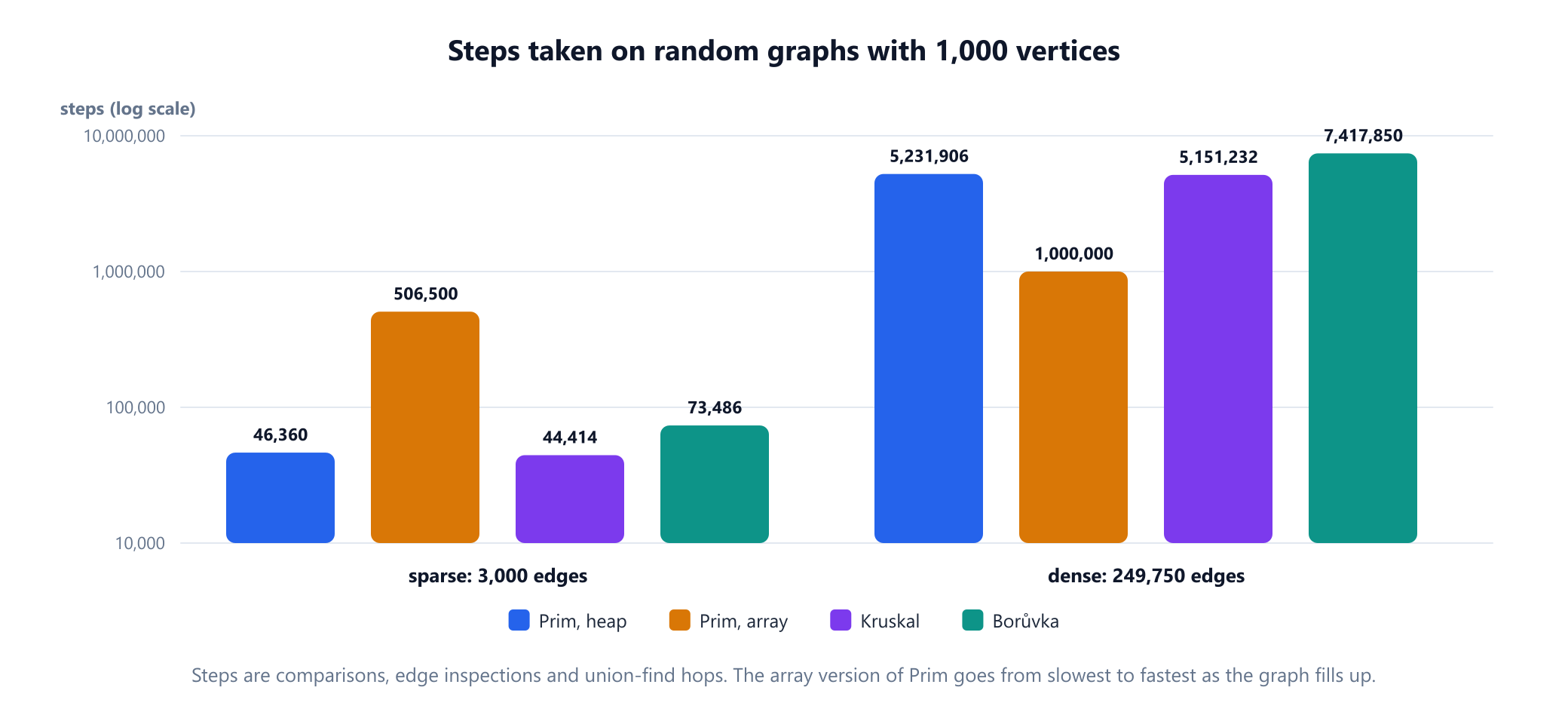
The results flip with density. On the sparse graph, Kruskal and Prim with a heap are within 5% of each other, Borůvka needs about 60% more, and array-based Prim is about 11 times slower, because it scans every remaining vertex even though each has few edges. On the dense graph the array version takes exactly 1,000,000 steps and wins by a factor of about five: it never has more than V candidates to look at, while the heap and the sort pay a logarithmic cost on nearly 250,000 edges.
These numbers count steps, not seconds. Sorting an array of numbers is very fast on real hardware, which often favours Kruskal, and the heap version here is the simple one that may hold several entries per vertex. A version that updates entries in place keeps the heap smaller at the price of more code. If the time matters, measure on your own data.
6. The shape of your input
Often the input decides before any complexity analysis does. The guide to graph representation compares the formats.
- A list of edges suits Kruskal directly: there is nothing to build except the union-find array.
- Edges already sorted, or weights that are small integers and can be counting-sorted, remove Kruskal's only expensive step. What remains is the union-find work, which is almost linear.
- An adjacency matrix, or distances you can compute on demand, such as points in a plane where every pair is an edge, suits array-based Prim. It never stores the edges at all, needing only
O(V)memory, while Kruskal would have to hold and sort aboutV2 / 2of them. - An edge list too large for memory favours Borůvka, which only needs repeated passes over the edges, and Kruskal variants such as filter-Kruskal, which avoid sorting edges that will clearly be rejected.
Kruskal's union-find structure is worth understanding on its own, and the guide to union-find covers it in depth.
7. Disconnected graphs and stopping early
The three methods also differ in what they do when the graph is not one piece, and in what they can tell you if you stop early.
Disconnected graphs. Prim only reaches the connected component of its start vertex; to cover the whole graph it has to be restarted in each component. Kruskal and Borůvka need no change: they simply run out of edges and return a minimum spanning forest, one tree per component.
Clustering. Kruskal's intermediate states are useful in themselves. Stop when k groups remain and those groups are the single-linkage clusters of the data: the division into k groups in which the closest pair of points from different groups is as far apart as possible.
PIPES = [('A', 'B', 3), ('A', 'C', 6), ('B', 'C', 4), ('B', 'D', 13), ('C', 'D', 7),
         ('C', 'E', 12), ('D', 'E', 2), ('D', 'F', 11), ('E', 'F', 8), ('E', 'G', 14),
         ('E', 'H', 5), ('F', 'G', 1), ('F', 'H', 15), ('G', 'H', 16)]

def kruskal_until(edges, groups_wanted):
    """Kruskal, stopped as soon as only groups_wanted groups remain."""
    parent = {x: x for u, v, _ in edges for x in (u, v)}
    def find(x):
        while parent[x] != x:
            parent[x] = parent[parent[x]]
            x = parent[x]
        return x
    count, tree = len(parent), []
    for u, v, w in sorted(edges, key=lambda e: e[2]):
        if count == groups_wanted:
            break
        if find(u) != find(v):
            parent[find(u)] = find(v)
            tree.append((u, v, w))
            count -= 1
    members = {}
    for x in sorted(parent):
        members.setdefault(find(x), []).append(x)
    return tree, sorted(''.join(m) for m in members.values())

print(kruskal_until(PIPES, 3)[1])              # three clusters of villages
# ['ABC', 'DEH', 'FG']
print(kruskal_until(PIPES, 2)[1])
# ['ABCDEH', 'FG']

# A graph in two pieces: drop every pipe between A to E and F, G, H.
split = [e for e in PIPES if not (set(e[:2]) & set('FGH')) or set(e[:2]) <= set('FGH')]
tree, parts = kruskal_until(split, 1)          # asks for 1 group, but only 2 can exist
print(parts, sum(w for *_, w in tree))
# ['ABCDE', 'FGH'] 32
Stopped at three groups, the program returns {A, B, C}, {D, E, H} and {F, G}, the same three that Borůvka's first round produced on this graph, although that agreement is a coincidence of the example. In the last run, with the pipes between the two halves removed, Kruskal returns a forest of two trees costing 32. Prim from A would stop after five villages and never see F, G or H.
8. Negative weights, maximum trees and directed graphs
- Negative weights are fine. Unlike Dijkstra's algorithm, none of the three is disturbed by them, because every spanning tree has exactly
V - 1edges. Adding the same constant to every weight raises the cost of every tree by the same amount and leaves the choice unchanged. Subtracting 10 from every pipe in the example, which makes most weights negative, gives the same tree. - Maximum spanning trees. Negate the weights, or sort in decreasing order. The most expensive spanning tree of the example costs 87.
- Bottlenecks. A minimum spanning tree also minimises its heaviest edge. In the example that edge is
E-Fat 8, and no spanning tree can avoid an edge of at least 8. - Directed graphs. None of the three works on directed graphs. The directed version of the problem, the minimum arborescence, needs the Chu-Liu/Edmonds algorithm.
9. Prim is not Dijkstra
Prim's algorithm and Dijkstra's look almost identical in code, and the difference is one line: Prim orders the queue by the weight of the single edge reaching a vertex, while Dijkstra orders it by the total distance from the source. They optimise different things and build different trees. The guide to Prim's algorithm compares them line by line.
On the example, Dijkstra's shortest-path tree from A uses A-C at 6 instead of B-C at 4. It costs 32 in total, against 30 for the minimum spanning tree. In return, every village is at least as close to A along it: C is 6 away instead of 7, H 20 instead of 21 and G 24 instead of 25. A minimum spanning tree minimises the cost of building the network and says nothing about the length of any single route.
10. A tangled history
The three names are misleading about who came first. The earliest algorithm is Borůvka's. In 1926 the Czech mathematician Otakar Borůvka published it after Jindřich Saxel, an employee of the West Moravian power company, asked him in the winter of 1925 how to electrify south-west Moravia as cheaply as possible. Vojtěch Jarník then described what is now called Prim's algorithm in 1930, in a paper written as a letter to Borůvka. Joseph Kruskal published his method in 1956, and Robert Prim rediscovered Jarník's algorithm in 1957 at Bell Laboratories, as did Edsger Dijkstra in 1959. Prim's algorithm is therefore sometimes called Jarník's algorithm or the DJP algorithm, although "Prim's" remains by far the most common name. Borůvka's method was itself rediscovered several times, and in some books it carries the name of Sollin, who presented it at a seminar in Paris in 1961 and never published it.
The fastest known methods have moved far from these classics. David Karger, Philip Klein and Robert Tarjan gave a randomized algorithm with expected linear time in 1995. Bernard Chazelle gave a deterministic algorithm in 2000 that runs in O(E α(E, V)), where α is the inverse Ackermann function, which is at most 4 for any graph that could ever be stored. In 2002 Seth Pettie and Vijaya Ramachandran found an algorithm that is provably optimal, although nobody knows what its running time actually is: it lies somewhere between linear and Chazelle's bound. Karger, Klein and Tarjan's algorithm uses Borůvka's rounds as a building block.
11. Where each one is used
- Network design. Laying cable, pipes or roads at least cost is the original application. Real designs add constraints, as the guide to network design shows, and the minimum spanning tree is the usual starting point.
- Clustering. Single-linkage clustering is Kruskal's algorithm stopped early, and it is why Kruskal is the usual choice for that job. The graph-based image segmentation method of Pedro Felzenszwalb and Daniel Huttenlocher processes edges in sorted order in the same way.
- Approximating harder problems. With nonnegative weights, a minimum spanning tree never costs more than the best travelling salesperson tour. Christofides' heuristic starts from one and guarantees a tour at most 1.5 times the optimum when distances obey the triangle inequality.
- Geometric data. When every pair of points is a candidate edge, the graph is complete and array-based Prim is the natural choice.
- Parallel computing. Each Borůvka round lets every group work independently, so it is the usual starting point for parallel algorithms, whereas Prim and Kruskal are inherently sequential.
12. Common mistakes
| Mistake | Why it is wrong | Fix |
|---|---|---|
| Using Prim on a disconnected graph and trusting the result | It only spans the start vertex's component | Restart it in each component, or use Kruskal |
| Assuming Prim with a heap is always best | On the dense graph the array version took five times fewer steps | Use the array version when E is close to V2 |
| Treating a minimum spanning tree as a set of shortest paths | In the example it reaches C at 7, but the shortest route costs 6 | Use Dijkstra for routes, a spanning tree for build cost |
| Testing for one exact tree when weights can tie | Several minimum trees can exist, and the input order picks one | Compare the total weight |
| Breaking ties inconsistently in Borůvka | Groups may choose edges that form a cycle | Compare by weight, then by a fixed edge order |
| Avoiding the algorithms because of negative weights | Negative weights do not affect any of the three | Run them unchanged |
| Running them on a directed graph | The cut property is about undirected edges | Use the Chu-Liu/Edmonds algorithm |
| Letting Kruskal scan every edge | The tree is complete after V - 1 accepted edges | Stop as soon as you have them |
13. Glossary
| Term | Meaning |
|---|---|
| Spanning tree | A tree that contains every vertex of the graph |
| Minimum spanning tree | A spanning tree of smallest total weight |
| Spanning forest | One spanning tree for each connected component |
| Cut property | The cheapest edge crossing any cut can be in a minimum spanning tree |
| Cycle property | The most expensive edge on any cycle can be left out |
| Union-find | A structure that tracks groups and merges them quickly |
| Priority queue | A structure that always returns the smallest key; usually a binary heap |
| Dense graph | A graph in which a large fraction of all vertex pairs are joined by edges |
| Sparse graph | A graph with few edges compared with V2, typically a small multiple of V |
| Single-linkage clustering | Grouping by repeatedly joining the two closest groups |
| Bottleneck edge | The heaviest edge of a tree |
| Arborescence | A directed tree in which every edge points away from one root |
14. Frequently asked questions
What is the difference between Prim's and Kruskal's algorithm?
Prim's algorithm grows one connected tree from a start vertex, always adding the cheapest edge that leaves it. Kruskal's algorithm sorts all the edges and takes them from cheapest up, skipping any edge that would close a cycle, so its tree starts as scattered fragments that merge. Both find a minimum spanning tree of the same total weight.
Which is better, Prim or Kruskal?
It depends on the graph. Kruskal is the natural choice for sparse graphs and for edges given as a list or already sorted. Prim with a plain array is the natural choice for dense graphs, since it runs in O(V squared) and does not need to sort the edges. On sparse graphs, Prim with a binary heap and Kruskal cost about the same.
Do Prim and Kruskal give the same minimum spanning tree?
If all edge weights are different, the minimum spanning tree is unique and both return exactly the same edges. If some weights are equal, there may be several minimum spanning trees, and the two algorithms can return different ones, but they always have the same total weight.
What is Borůvka's algorithm?
Borůvka's algorithm works in rounds. In each round, every group of connected vertices picks its cheapest edge to another group, and all those edges are added at once. The number of groups at least halves each round, so there are at most log2 V rounds and the running time is O(E log V). Because the groups work independently, it is well suited to parallel computing.
Can Prim and Kruskal handle negative edge weights?
Yes. Unlike Dijkstra's algorithm, Prim, Kruskal and Borůvka all work correctly with negative weights. Every spanning tree has exactly V - 1 edges, so adding the same constant to every weight changes the cost of every tree equally and does not change which tree is cheapest.
What is the difference between Prim's algorithm and Dijkstra's algorithm?
Their code is almost identical, but Prim orders vertices by the weight of the single edge reaching them, while Dijkstra orders them by total distance from the source. Prim builds the tree of least total weight. Dijkstra builds a tree of shortest paths from one source, which can cost more in total but gives shorter routes from that source.
15. References
The algorithms, bounds and attributions above come from these sources, listed in chronological order.
- Borůvka, O. (1926). "O jistém problému minimálním." Práce Moravské přírodovědecké společnosti 3, 37 to 58.
- Jarník, V. (1930). "O jistém problému minimálním (Z dopisu panu O. Borůvkovi)." Práce Moravské přírodovědecké společnosti 6, 57 to 63.
- Kruskal, J. B. (1956). "On the Shortest Spanning Subtree of a Graph and the Traveling Salesman Problem." Proceedings of the American Mathematical Society 7(1), 48 to 50.
- Prim, R. C. (1957). "Shortest Connection Networks and Some Generalizations." Bell System Technical Journal 36(6), 1389 to 1401.
- Dijkstra, E. W. (1959). "A Note on Two Problems in Connexion with Graphs." Numerische Mathematik 1, 269 to 271.
- Chu, Y.-J. and Liu, T.-H. (1965). "On the Shortest Arborescence of a Directed Graph." Scientia Sinica 14, 1396 to 1400.
- Edmonds, J. (1967). "Optimum Branchings." Journal of Research of the National Bureau of Standards 71B, 233 to 240.
- Gower, J. C. and Ross, G. J. S. (1969). "Minimum Spanning Trees and Single Linkage Cluster Analysis." Journal of the Royal Statistical Society, Series C 18(1), 54 to 64.
- Tarjan, R. E. (1975). "Efficiency of a Good But Not Linear Set Union Algorithm." Journal of the ACM 22(2), 215 to 225.
- Christofides, N. (1976). Worst-Case Analysis of a New Heuristic for the Travelling Salesman Problem. Report 388. Pittsburgh: Carnegie Mellon University.
- Graham, R. L. and Hell, P. (1985). "On the History of the Minimum Spanning Tree Problem." Annals of the History of Computing 7(1), 43 to 57.
- Fredman, M. L. and Tarjan, R. E. (1987). "Fibonacci Heaps and Their Uses in Improved Network Optimization Algorithms." Journal of the ACM 34(3), 596 to 615.
- Karger, D. R., Klein, P. N. and Tarjan, R. E. (1995). "A Randomized Linear-Time Algorithm to Find Minimum Spanning Trees." Journal of the ACM 42(2), 321 to 328.
- Chazelle, B. (2000). "A Minimum Spanning Tree Algorithm with Inverse-Ackermann Type Complexity." Journal of the ACM 47(6), 1028 to 1047.
- Nešetřil, J., Milková, E. and Nešetřilová, H. (2001). "Otakar Borůvka on Minimum Spanning Tree Problem." Discrete Mathematics 233(1 to 3), 3 to 36.
- Pettie, S. and Ramachandran, V. (2002). "An Optimal Minimum Spanning Tree Algorithm." Journal of the ACM 49(1), 16 to 34.
- Felzenszwalb, P. F. and Huttenlocher, D. P. (2004). "Efficient Graph-Based Image Segmentation." International Journal of Computer Vision 59(2), 167 to 181.
- Kleinberg, J. and Tardos, É. (2005). Algorithm Design. Boston: Addison-Wesley.
- Bader, D. A. and Cong, G. (2006). "Fast Shared-Memory Algorithms for Computing the Minimum Spanning Forest of Sparse Graphs." Journal of Parallel and Distributed Computing 66(11), 1366 to 1378.
- Cormen, T. H., Leiserson, C. E., Rivest, R. L. and Stein, C. (2009). Introduction to Algorithms, 3rd edition. Cambridge, MA: MIT Press.
- Osipov, V., Sanders, P. and Singler, J. (2009). "The Filter-Kruskal Minimum Spanning Tree Algorithm." In Proceedings of the 11th Workshop on Algorithm Engineering and Experiments, 52 to 61.
Watch the tree grow
Build the eight villages in the visualizer and run Prim from A. Then run Kruskal on the same graph and compare the order in which the edges appear.
Open the visualizer