
Table of Contents
- 1. The short answer
- 2. One graph, three answers
- 3. What each algorithm does
- 4. Why Dijkstra breaks on negative edges
- 5. Negative cycles
- 6. Speed: which one is faster, and when
- 7. All pairs with negative edges: Johnson's algorithm
- 8. When none of the three is the best choice
- 9. Memory and recovering the paths
- 10. Where each one is used
- 11. Still an active research area
- 12. Common mistakes
- 13. Glossary
- 14. Frequently asked questions
- 15. References
1. The short answer
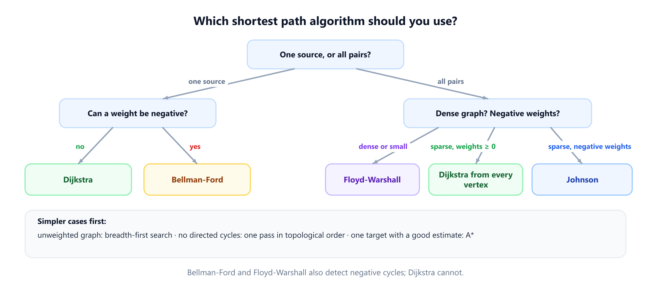
Dijkstra's algorithm, the Bellman-Ford algorithm and the Floyd-Warshall algorithm all find shortest paths in a weighted graph, but they answer different questions under different conditions. Two questions decide between them: do you need distances from one source or between every pair of vertices, and can an edge have a negative weight?
| Dijkstra | Bellman-Ford | Floyd-Warshall | |
|---|---|---|---|
| Answers | One source to every vertex | One source to every vertex | Every pair of vertices |
| Negative edge weights | No: gives wrong answers | Yes | Yes |
| Detects negative cycles | No | Yes | Yes |
| Time | O((V + E) log V) with a binary heap | O(V E) | O(V3) |
| Memory | O(V) | O(V) | O(V2) |
| Strategy | Greedy: settle the closest vertex | Repeat: relax every edge | Dynamic programming over stopovers |
| Use it when | Weights are nonnegative, which covers most road, network and game maps | Some weights are negative, or a negative cycle must be detected | You need all distances in a small or dense graph |
Here V is the number of vertices and E the number of edges. In one sentence: use Dijkstra by default, switch to Bellman-Ford when weights can be negative, and use Floyd-Warshall when you need the whole distance table of a graph with at most a few hundred vertices. When you need all pairs in a large sparse graph with negative edges, Johnson's algorithm in section 7 combines the first two. The rest of this guide runs all three on the same graph and shows where each one wins and where each one breaks.
2. One graph, three answers
The running example is a small directed graph with six vertices, seven edges and one negative edge, B → A with weight -4. Think of the weights as costs: a negative cost is a refund, such as a toll road that pays you to take it, or a step in a chemical process that releases energy.
S → A  3      S → B  6      A → C  4      B → A  -4
C → T  2      B → D  3      D → T  4

6 vertices, 7 edges, no cycles; source S
The cheapest route from S to T is S, B, A, C, T, with cost 6 - 4 + 4 + 2 = 8. It starts with the more expensive first step, to B, and earns it back on the refund. The program below implements the three algorithms in their standard textbook form and runs them from S.
import heapq
INF = float('inf')

def graph(edges):
    adj = {}
    for u, v, w in edges:
        adj.setdefault(u, []).append((v, w))
        adj.setdefault(v, [])
    return adj

def dijkstra(adj, s):
    """Greedy: settle the closest unsettled vertex, never revisit it."""
    dist = {v: INF for v in adj}
    dist[s] = 0
    done, heap = set(), [(0, s)]
    while heap:
        d, u = heapq.heappop(heap)
        if u in done:
            continue                      # stale heap entry
        done.add(u)
        for v, w in adj[u]:
            if v not in done and d + w < dist[v]:
                dist[v] = d + w
                heapq.heappush(heap, (dist[v], v))
    return dist

def bellman_ford(adj, s):
    """Relax every edge, round after round, until nothing changes."""
    dist = {v: INF for v in adj}
    dist[s] = 0
    for _ in range(len(adj) - 1):
        changed = False
        for u in adj:
            for v, w in adj[u]:
                if dist[u] + w < dist[v]:
                    dist[v] = dist[u] + w
                    changed = True
        if not changed:
            break
    return dist

def floyd_warshall(adj):
    """All pairs: allow the vertices as stopovers one at a time."""
    d = {u: {v: 0 if u == v else INF for v in adj} for u in adj}
    for u in adj:
        for v, w in adj[u]:
            d[u][v] = min(d[u][v], w)
    for k in adj:
        for i in adj:
            for j in adj:
                if d[i][k] + d[k][j] < d[i][j]:
                    d[i][j] = d[i][k] + d[k][j]
    return d

G = graph([('S', 'A', 3), ('S', 'B', 6), ('A', 'C', 4), ('B', 'A', -4),
           ('C', 'T', 2), ('B', 'D', 3), ('D', 'T', 4)])
dj, bf, fw = dijkstra(G, 'S'), bellman_ford(G, 'S'), floyd_warshall(G)['S']
for v in G:
    print(v, dj[v], bf[v], fw[v], '' if dj[v] == bf[v] else '<- Dijkstra is wrong')
# S 0 0 0
# A 3 2 2 <- Dijkstra is wrong
# B 6 6 6
# C 7 6 6 <- Dijkstra is wrong
# T 9 8 8 <- Dijkstra is wrong
# D 9 9 9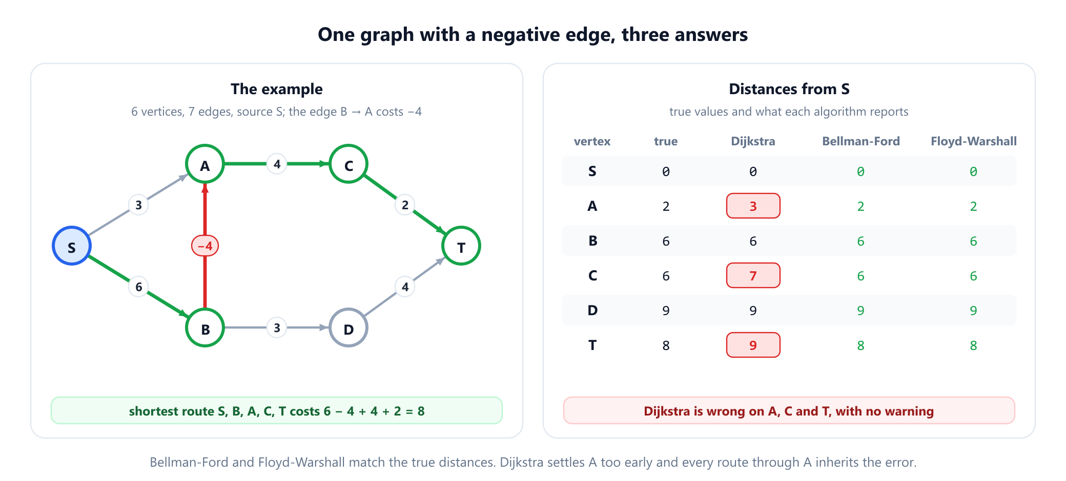
Bellman-Ford and Floyd-Warshall return the true distances. Dijkstra reports 3 for A, 7 for C and 9 for T, all too high, and it raises no error: the wrong answers look exactly like right ones. Section 4 explains why. On a graph with nonnegative weights all three would agree, and the only difference would be speed.
3. What each algorithm does
All three algorithms are built from one operation, relaxation. Each vertex v carries a tentative distance dist[v], which starts at infinity, or 0 for the source. Relaxing the edge u → v with weight w asks whether going through u is cheaper, and if so records it:
if dist[u] + w < dist[v]:
    dist[v] = dist[u] + w
A tentative distance only ever goes down, and it is always the cost of some real route. The algorithms differ only in which edges they relax and in what order.
- Dijkstra keeps the unsettled vertices in a priority queue. It repeatedly takes the one with the smallest tentative distance, declares that distance final, and relaxes its outgoing edges. Each vertex is settled once and each edge relaxed once. Edsger Dijkstra designed it in 1956, in about twenty minutes by his own account, and published it in 1959. The guide to Dijkstra's algorithm traces it step by step.
- Bellman-Ford makes no choices. It relaxes every edge, in any fixed order, and repeats. A shortest path without cycles has at most
V - 1edges, and after roundievery shortest path with at mostiedges has been found, soV - 1rounds are always enough. The name joins Richard Bellman, who published the round-based method in 1958, and Lester Ford, whose 1956 paper gave the general rule of relaxing edges until nothing improves. Alfonso Shimbel and Edward Moore found equivalent methods in the same years. The guide to the Bellman-Ford algorithm proves the bound. - Floyd-Warshall computes the whole table at once. It allows the vertices as stopovers one at a time: after step
k, entry[i][j]holds the cheapest route fromitojwhose intermediate vertices all come from the firstk. Three nested loops and one line of arithmetic. Bernard Roy in 1959 and Stephen Warshall in 1962 published the same scheme for reachability, and Robert Floyd adapted it to shortest paths in 1962. The guide to the Floyd-Warshall algorithm derives the recurrence.
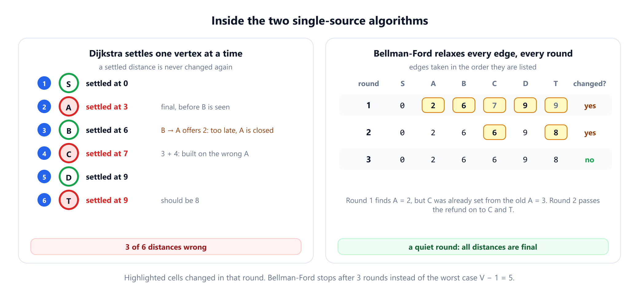
On the example, Bellman-Ford visits the edges in the order they were listed. Its first round already lowers A to 2 when it reaches the edges out of B, but by then it has used the old value 3 to set C = 7. The second round carries the improvement on to C = 6 and T = 8. The third round changes nothing, so the algorithm stops early instead of running all V - 1 = 5 rounds. How many rounds are needed depends on the edge order, but never exceeds V - 1.
4. Why Dijkstra breaks on negative edges
Dijkstra's speed comes from one promise: when a vertex leaves the priority queue, its distance is final. The promise rests on an argument that needs nonnegative weights. Suppose u is the closest unsettled vertex. Any other route to u has to leave the settled region through some unsettled vertex x, which is already at least as far as u, and the rest of the route can only add cost. With a negative edge, the rest of the route can subtract cost, and the argument collapses.
That is exactly what happens in the example. Dijkstra settles S at 0, then A at 3, because 3 is less than B's 6. When B is settled and its edge to A offers 6 - 4 = 2, A is already final and the improvement is thrown away. Everything built on top of A inherits the error: C is settled at 3 + 4 = 7 instead of 6, and T at 9 instead of 8.
Two tempting fixes do not work:
- Adding a constant to every weight. Adding 4 makes every weight nonnegative, but it charges 4 for every edge, so routes with more edges are penalised more. On the shifted graph Dijkstra finds
S, A, C, T, with shifted cost 21 against 24 for the true shortest routeS, B, A, C, T, which has one edge more. Back in the original weights that route costs 9, not 8. Johnson's algorithm in section 7 shows the reweighting that does work. - Letting settled vertices reopen. If a vertex may re-enter the queue whenever its distance drops, the algorithm becomes correct for negative edges as long as there is no negative cycle. But the promise that made it fast is gone, and Donald Johnson showed in 1973 that Dijkstra's algorithm adapted in this way to allow negative edges can take exponential time, on the order of
n 2nsteps on a family of graphs withnvertices. At that point Bellman-Ford's guaranteedO(V E)is the safer choice.
With nonnegative weights, none of this arises, and Dijkstra is correct and the fastest of the three. Zero weights are fine: the argument only needs that no edge decreases the cost.
5. Negative cycles
A negative cycle is a cycle whose weights add up to less than zero. If one can be reached from the source and can reach the target, there is no shortest route at all: going round the cycle once more is always cheaper. The distance is minus infinity, and an algorithm should report the cycle rather than a number. Add the edge C → B with weight -5 to the example and the cycle B, A, C, B costs -4 + 4 - 5 = -5.
- Bellman-Ford detects it with one extra round. Without a negative cycle, nothing can improve after
V - 1rounds; if roundVstill lowers a distance, a negative cycle exists, and following the parent pointers back from the changed vertex leads onto it. - Floyd-Warshall detects it on the diagonal. Entry
[v][v]starts at 0 and can only become negative if there is a closed route throughvwith negative total weight. So a negative cycle exists exactly when some diagonal entry ends below zero. Once that happens, the other entries are no longer meaningful distances, and Stefan Hougardy showed in 2010 that they can grow exponentially large, so it is safest to check the diagonal inside the loop and stop as soon as an entry turns negative. - Dijkstra cannot detect one. It assumes the situation away.
INF = float('inf')

def graph(edges):
    adj = {}
    for u, v, w in edges:
        adj.setdefault(u, []).append((v, w))
        adj.setdefault(v, [])
    return adj

def negative_cycle(adj):
    """Bellman-Ford from a virtual source joined to every vertex at cost 0.
    Returns a negative cycle as a list of vertices, or None."""
    dist = {v: 0 for v in adj}
    parent = {v: None for v in adj}
    for _ in range(len(adj)):                  # one round more than usual
        last = None
        for u in adj:
            for v, w in adj[u]:
                if dist[u] + w < dist[v]:
                    dist[v], parent[v], last = dist[u] + w, u, v
        if last is None:
            return None                        # a quiet round: no negative cycle
    for _ in range(len(adj)):                  # step back far enough to land on the cycle
        last = parent[last]
    cycle, v = [last], parent[last]
    while v != last:                           # follow parents once round the cycle
        cycle.append(v)
        v = parent[v]
    cycle.reverse()                            # parents point backwards
    return cycle + cycle[:1]

def floyd_warshall_diagonal(adj):
    """Vertices whose distance to themselves comes out negative."""
    d = {u: {v: 0 if u == v else INF for v in adj} for u in adj}
    for u in adj:
        for v, w in adj[u]:
            d[u][v] = min(d[u][v], w)
    for k in adj:
        for i in adj:
            for j in adj:
                if d[i][k] + d[k][j] < d[i][j]:
                    d[i][j] = d[i][k] + d[k][j]
    return [v for v in adj if d[v][v] < 0]

edges = [('S', 'A', 3), ('S', 'B', 6), ('A', 'C', 4), ('B', 'A', -4),
         ('C', 'T', 2), ('B', 'D', 3), ('D', 'T', 4)]
print(negative_cycle(graph(edges)))
# None
bad = graph(edges + [('C', 'B', -5)])          # B -> A -> C -> B costs -4 + 4 - 5 = -5
print(negative_cycle(bad))
# ['C', 'B', 'A', 'C']
print(floyd_warshall_diagonal(bad))
# ['A', 'B', 'C']
The function starts Bellman-Ford from a virtual source joined to every vertex at cost 0, so it finds a negative cycle anywhere in the graph, not only one reachable from S. On the original example a round eventually changes nothing and it returns None. With the extra edge it returns the cycle C, B, A, C, the same cycle written from a different start, and Floyd-Warshall flags A, B and C on its diagonal. In testing on thousands of random graphs, the diagonal flagged a negative cycle exactly when one existed, but did not always flag every vertex that can reach one, so use it as a yes-or-no test.
One trap catches many people. In an undirected graph, an edge can be walked both ways, so a single edge with negative weight is already a negative cycle: u, v, u. Bellman-Ford run on the directed version of an undirected graph will therefore report a negative cycle whenever any edge is negative, a pitfall that Sedgewick and Wayne's Algorithms spells out. Shortest simple paths with negative weights in undirected graphs need different, more involved methods.
6. Speed: which one is faster, and when
For a single source the order is clear whenever Dijkstra applies: O((V + E) log V) with a binary heap against Bellman-Ford's O(V E). On a graph with 10,000 vertices and 50,000 edges, that is roughly a million heap steps against up to 500 million edge relaxations. Floyd-Warshall is not a single-source method, and running it for one source wastes almost all its work.
For all pairs the comparison is closer, because the alternatives are to run a single-source algorithm from every vertex:
| All-pairs method | Time | Negative edges | Best for |
|---|---|---|---|
| Dijkstra from every vertex | O(V (V + E) log V) | No | Sparse graphs, nonnegative weights |
| Bellman-Ford from every vertex | O(V2 E) | Yes | Almost never |
| Floyd-Warshall | O(V3) | Yes | Dense or small graphs |
| Johnson's algorithm | O(V E + V (V + E) log V) | Yes | Sparse graphs with negative edges |
Asymptotic bounds hide constants, so the program below counts the basic steps each method actually performs on two random directed graphs with 100 vertices: a sparse one with 300 edges and a dense one with 4,950, half of all possible edges. For Dijkstra it counts edge checks and heap operations separately, since a heap operation costs about log V steps.
import heapq, random
INF = float('inf')

def random_graph(n, m, seed):
    """n vertices, m distinct directed edges with weights 1..100."""
    rnd = random.Random(seed)
    pairs = rnd.sample([(u, v) for u in range(n) for v in range(n) if u != v], m)
    adj = {v: [] for v in range(n)}
    for u, v in pairs:
        adj[u].append((v, rnd.randint(1, 100)))
    return adj

def all_pairs_dijkstra(adj):
    """Dijkstra from every vertex. Counts edge checks and heap operations."""
    checks = heap_ops = 0
    for s in adj:
        dist, heap = {v: INF for v in adj}, [(0, s)]
        dist[s] = 0
        while heap:
            d, u = heapq.heappop(heap)
            heap_ops += 1
            if d > dist[u]:
                continue
            for v, w in adj[u]:
                checks += 1
                if d + w < dist[v]:
                    dist[v] = d + w
                    heapq.heappush(heap, (dist[v], v))
                    heap_ops += 1
    return checks, heap_ops

def all_pairs_bellman_ford(adj):
    """Bellman-Ford from every vertex, stopping early when a round changes nothing."""
    m, checks = sum(len(a) for a in adj.values()), 0
    for s in adj:
        dist = {v: INF for v in adj}
        dist[s] = 0
        for _ in range(len(adj) - 1):
            changed = False
            for u in adj:
                for v, w in adj[u]:
                    if dist[u] + w < dist[v]:
                        dist[v], changed = dist[u] + w, True
            checks += m
            if not changed:
                break
    return checks

n = 100
for name, m in [('sparse', 3 * n), ('dense', n * (n - 1) // 2)]:
    adj = random_graph(n, m, seed=1)
    checks, heap_ops = all_pairs_dijkstra(adj)
    print(f'{name:6} E={m:4}  Dijkstra x V: {checks:7,} checks + {heap_ops:6,} heap ops   '
          f'Bellman-Ford x V: {all_pairs_bellman_ford(adj):9,}   Floyd-Warshall: {n ** 3:,}')
# sparse E= 300  Dijkstra x V:  27,565 checks + 21,388 heap ops   Bellman-Ford x V:   226,200   Floyd-Warshall: 1,000,000
# dense  E=4950  Dijkstra x V: 495,000 checks + 64,770 heap ops   Bellman-Ford x V: 2,712,600   Floyd-Warshall: 1,000,000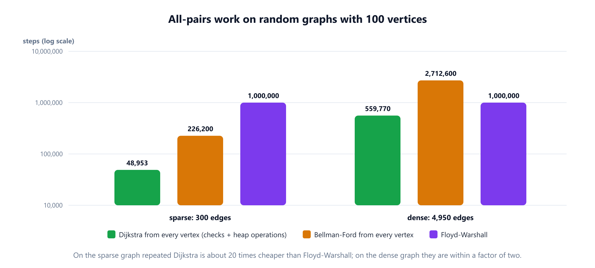
On the sparse graph, Dijkstra from every vertex needs about 49,000 steps against Floyd-Warshall's fixed 1,000,000, a factor of about 20. On the dense graph the gap almost closes, and once the heap's logarithmic cost per operation is counted, Floyd-Warshall's simple inner loop, which touches memory in order and needs no priority queue, often wins in practice. Bellman-Ford from every vertex is the slowest in both cases, even with early stopping. The rule of thumb: below a few hundred vertices, or when most pairs of vertices are joined by an edge, use Floyd-Warshall for its simplicity; on large sparse graphs, use Dijkstra or Johnson from every vertex.
7. All pairs with negative edges: Johnson's algorithm
Donald Johnson's algorithm of 1977 gets the best of both. It runs Bellman-Ford once to compute a number h(v) for every vertex, the distance from a virtual source joined to all vertices at cost 0. It then replaces each weight by
w'(u, v) = w(u, v) + h(u) - h(v)Because h satisfies h(v) ≤ h(u) + w(u, v) for every edge, every new weight is nonnegative. And along any route from s to t the terms telescope, so every route's cost changes by the same amount, h(s) - h(t). Shortest routes stay shortest, and Dijkstra can now be run from every vertex. Unlike adding a constant, this reweighting does not depend on how many edges a route has.
import heapq
INF = float('inf')

def graph(edges):
    adj = {}
    for u, v, w in edges:
        adj.setdefault(u, []).append((v, w))
        adj.setdefault(v, [])
    return adj

def dijkstra(adj, s):
    dist, heap = {v: INF for v in adj}, [(0, s)]
    dist[s] = 0
    while heap:
        d, u = heapq.heappop(heap)
        if d > dist[u]:
            continue
        for v, w in adj[u]:
            if d + w < dist[v]:
                dist[v] = d + w
                heapq.heappush(heap, (dist[v], v))
    return dist

def johnson(adj):
    """All pairs with negative edges: one Bellman-Ford, then Dijkstra from every vertex."""
    h = {v: 0 for v in adj}                    # distances from a virtual source
    for _ in range(len(adj)):
        for u in adj:
            for v, w in adj[u]:
                h[v] = min(h[v], h[u] + w)
    for u in adj:
        for v, w in adj[u]:
            if h[u] + w < h[v]:
                raise ValueError('negative cycle')
    # reweight: every edge becomes nonnegative, every path changes by h[s] - h[t]
    lifted = {u: [(v, w + h[u] - h[v]) for v, w in adj[u]] for u in adj}
    return {s: {t: d - h[s] + h[t] for t, d in dijkstra(lifted, s).items()} for s in adj}, lifted

G = graph([('S', 'A', 3), ('S', 'B', 6), ('A', 'C', 4), ('B', 'A', -4),
           ('C', 'T', 2), ('B', 'D', 3), ('D', 'T', 4)])
dist, lifted = johnson(G)
print({u: [(v, w) for v, w in lifted[u]] for u in ('S', 'A', 'B')})
# {'S': [('A', 7), ('B', 6)], 'A': [('C', 0)], 'B': [('A', 0), ('D', 3)]}
print(dist['S'])
# {'S': 0, 'A': 2, 'B': 6, 'C': 6, 'T': 8, 'D': 9}
print(dist['B'])
# {'S': inf, 'A': -4, 'B': 0, 'C': 0, 'T': 2, 'D': 3}
In the example, h(A) = -4 and every other vertex gets 0. The negative edge B → A becomes 0, S → A rises from 3 to 7 and A → C falls from 4 to 0, and Dijkstra on the new weights, corrected back by h, gives the true distances from every source, including the row for B with its negative entry -4. If Bellman-Ford finds a negative cycle in the first step, Johnson's algorithm stops and reports it.
8. When none of the three is the best choice
Some graphs have structure that a simpler or faster method can exploit:
- Unweighted graphs. If every edge counts as 1, breadth-first search finds all distances from a source in
O(V + E). Dijkstra would give the same answer more slowly. See BFS vs DFS. - Acyclic graphs. In a directed acyclic graph, process the vertices in topological order and relax each vertex's outgoing edges once. That takes
O(V + E)and works with negative weights. The example graph has no cycles, so this method would have solved it in a single pass. - Weights 0 and 1 only. A double-ended queue replaces the priority queue: 0-weight edges go to the front and 1-weight edges to the back, which gives linear time.
- One source and one target with a good estimate. A* search adds an estimate of the remaining distance to Dijkstra's priority and explores far fewer vertices on maps. See the A* search algorithm.
9. Memory and recovering the paths
Distances are often not enough: you want the route itself. Dijkstra and Bellman-Ford store one parent per vertex, the vertex the best route arrived from, and the route to t is read backwards from t. That costs O(V) extra memory. Floyd-Warshall needs a full V by V table of "next hop" entries alongside its distance table, so its memory is O(V2). For 10,000 vertices with 8-byte entries, the distance table alone takes about 800 megabytes, and the next-hop table adds as much again. Memory, more than time, is usually what rules Floyd-Warshall out on large graphs.
10. Where each one is used
- Dijkstra is the default wherever costs are physical: road navigation, flight connections and the link-state routing protocols of the internet, such as OSPF, in which every router computes shortest paths over a map of the network.
- Bellman-Ford suits settings where each node only knows its neighbours. Distance-vector routing protocols such as RIP repeat its relaxation step across the network, with each router updating its table from its neighbours' tables. Its ability to find negative cycles is used to detect currency arbitrage: with weights
-log(rate), a sequence of trades that ends with more money than it started is exactly a negative cycle. - Floyd-Warshall fills complete distance tables for small graphs: distance matrices for clustering or the travelling salesperson problem, and transitive closure, the question of which vertices can reach which, which is the version Warshall published.
11. Still an active research area
Shortest paths are one of the oldest problems in algorithms, and the bounds are still moving. In 2022, Aaron Bernstein, Danupon Nanongkai and Christian Wulff-Nilsen showed that single-source shortest paths with negative integer weights can be solved in nearly linear time, far below Bellman-Ford's O(V E). In 2024, Bernhard Haeupler and coauthors proved that Dijkstra's algorithm with a suitably designed heap is universally optimal for ordering vertices by distance: on every fixed graph, its worst case over all edge weights is within a constant factor of the best any algorithm can do. And in 2025, Ran Duan and coauthors gave a deterministic algorithm for directed graphs with nonnegative weights that runs in O(E log2/3 V) time, beating Dijkstra's O(E + V log V) on sparse graphs. It escapes what was long called the sorting barrier because, unlike Dijkstra, it does not produce the vertices in order of distance. Each of the three papers won a best paper award. None of these has yet replaced the three classics in everyday code, where simplicity and small constants matter more.
12. Common mistakes
| Mistake | Why it is wrong | Fix |
|---|---|---|
| Running Dijkstra on a graph with negative edges | Settled vertices are never revisited; the example gets A, C and T wrong | Use Bellman-Ford, or Johnson for all pairs |
| Adding a constant to make weights nonnegative | It penalises routes with more edges and changes which route is shortest | Reweight with potentials, as Johnson's algorithm does |
| Ignoring negative cycles | Distances are minus infinity; any number reported is meaningless | Run one extra Bellman-Ford round, or check the Floyd-Warshall diagonal |
| A negative edge in an undirected graph | Walking it there and back is a negative cycle | Treat the problem as shortest simple paths, which needs other methods |
| Using Floyd-Warshall for one source | O(V3) work for one row of the table | Use Dijkstra or Bellman-Ford |
| Using Floyd-Warshall on a huge sparse graph | The V by V table may not fit in memory | Run Dijkstra or Johnson from the sources you need |
Using INF + w with a fixed large integer | Infinity plus a negative weight looks like a real distance, or overflows | Skip relaxations from vertices still at infinity |
Running Bellman-Ford for exactly V rounds and trusting the result | Round V is the test round; changes there mean a negative cycle | Run V - 1 rounds, then check once more |
13. Glossary
| Term | Meaning |
|---|---|
| Single-source shortest paths | Distances from one vertex to every other vertex |
| All-pairs shortest paths | Distances between every ordered pair of vertices |
| Relaxation | Checking whether a route through one more edge is cheaper, and recording it if so |
| Settled vertex | In Dijkstra's algorithm, a vertex whose distance has been declared final |
| Negative edge | An edge with a weight below zero |
| Negative cycle | A cycle whose weights add up to less than zero |
| Priority queue | A structure that always returns the smallest key; usually a binary heap |
| Potential | A number h(v) per vertex used to reweight edges without changing which routes are shortest |
| Dense graph | A graph in which a large fraction of all vertex pairs are joined by edges |
| Sparse graph | A graph with few edges compared with V2, typically a small multiple of V |
| Transitive closure | The table of which vertices can reach which |
14. Frequently asked questions
What is the difference between Dijkstra, Bellman-Ford and Floyd-Warshall?
Dijkstra and Bellman-Ford compute distances from one source vertex to every other vertex, while Floyd-Warshall computes the distance between every pair of vertices. Dijkstra is the fastest but requires nonnegative edge weights. Bellman-Ford handles negative weights and detects negative cycles in O(VE) time. Floyd-Warshall also handles negative weights and detects negative cycles, in O(V cubed) time and O(V squared) memory.
Why does Dijkstra not work with negative weights?
Dijkstra declares a vertex's distance final as soon as it is the closest unsettled vertex, and never revisits it. That is only safe if no later edge can lower the cost. A negative edge can do exactly that, so Dijkstra may finalise a vertex too early and report distances that are too high, without any warning.
Is Bellman-Ford slower than Dijkstra?
Yes, whenever both apply. Bellman-Ford runs in O(VE) time, while Dijkstra with a binary heap runs in O((V + E) log V). On a graph with 10,000 vertices and 50,000 edges that is up to 500 million edge relaxations against about a million heap steps. Use Bellman-Ford only when weights can be negative or a negative cycle must be detected.
When should I use Floyd-Warshall instead of running Dijkstra from every vertex?
Use Floyd-Warshall when you need all pairs of distances in a small graph, up to a few hundred vertices, or in a dense graph in which most pairs of vertices are joined by edges, and also when weights can be negative. On large sparse graphs, running Dijkstra from every vertex, or Johnson's algorithm if weights can be negative, is much faster and uses far less memory.
How do you detect a negative cycle?
Run Bellman-Ford for V - 1 rounds and then one more: if the extra round still lowers any distance, a negative cycle exists, and following parent pointers from the changed vertex leads onto it. With Floyd-Warshall, a negative cycle exists exactly when some entry on the diagonal of the final distance matrix is negative. Dijkstra cannot detect negative cycles.
What is Johnson's algorithm?
Johnson's algorithm computes all-pairs shortest paths in sparse graphs with negative edges. It runs Bellman-Ford once to get a potential h(v) for every vertex, reweights each edge to w(u, v) + h(u) - h(v), which is never negative and keeps the same shortest paths, and then runs Dijkstra from every vertex. Its running time is O(VE + V(V + E) log V) with a binary heap.
15. References
The algorithms, bounds and attributions above come from these sources, listed in chronological order.
- Shimbel, A. (1955). "Structure in Communication Nets." In Proceedings of the Symposium on Information Networks, 199 to 203. Brooklyn: Polytechnic Press of the Polytechnic Institute of Brooklyn.
- Ford, L. R. (1956). Network Flow Theory. Paper P-923. Santa Monica: RAND Corporation.
- Bellman, R. (1958). "On a Routing Problem." Quarterly of Applied Mathematics 16(1), 87 to 90.
- Dijkstra, E. W. (1959). "A Note on Two Problems in Connexion with Graphs." Numerische Mathematik 1, 269 to 271.
- Moore, E. F. (1959). "The Shortest Path Through a Maze." In Proceedings of an International Symposium on the Theory of Switching, 285 to 292. Cambridge, MA: Harvard University Press.
- Roy, B. (1959). "Transitivité et connexité." Comptes Rendus de l'Académie des Sciences 249, 216 to 218.
- Floyd, R. W. (1962). "Algorithm 97: Shortest Path." Communications of the ACM 5(6), 345.
- Warshall, S. (1962). "A Theorem on Boolean Matrices." Journal of the ACM 9(1), 11 to 12.
- Johnson, D. B. (1973). "A Note on Dijkstra's Shortest Path Algorithm." Journal of the ACM 20(3), 385 to 388.
- Johnson, D. B. (1977). "Efficient Algorithms for Shortest Paths in Sparse Networks." Journal of the ACM 24(1), 1 to 13.
- Fredman, M. L. and Tarjan, R. E. (1987). "Fibonacci Heaps and Their Uses in Improved Network Optimization Algorithms." Journal of the ACM 34(3), 596 to 615.
- Moy, J. (1998). "OSPF Version 2." RFC 2328. Internet Engineering Task Force.
- Malkin, G. (1998). "RIP Version 2." RFC 2453. Internet Engineering Task Force.
- Cormen, T. H., Leiserson, C. E., Rivest, R. L. and Stein, C. (2009). Introduction to Algorithms, 3rd edition. Cambridge, MA: MIT Press.
- Frana, P. L. and Misa, T. J. (2010). "An Interview with Edsger W. Dijkstra." Communications of the ACM 53(8), 41 to 47.
- Hougardy, S. (2010). "The Floyd-Warshall Algorithm on Graphs with Negative Cycles." Information Processing Letters 110(8 to 9), 279 to 281.
- Sedgewick, R. and Wayne, K. (2011). Algorithms, 4th edition. Upper Saddle River, NJ: Addison-Wesley.
- Schrijver, A. (2012). "On the History of the Shortest Path Problem." Documenta Mathematica, Extra Volume ISMP, 155 to 167.
- Bernstein, A., Nanongkai, D. and Wulff-Nilsen, C. (2022). "Negative-Weight Single-Source Shortest Paths in Near-linear Time." Proceedings of the 63rd IEEE Symposium on Foundations of Computer Science, 600 to 611.
- Haeupler, B., Hladík, R., Rozhoň, V., Tarjan, R. E. and Tětek, J. (2024). "Universal Optimality of Dijkstra via Beyond-Worst-Case Heaps." Proceedings of the 65th IEEE Symposium on Foundations of Computer Science, 2099 to 2130.
- Duan, R., Mao, J., Mao, X., Shu, X. and Yin, L. (2025). "Breaking the Sorting Barrier for Directed Single-Source Shortest Paths." Proceedings of the 57th ACM Symposium on Theory of Computing, 36 to 44.
Watch the negative edge do its work
Build the example in the visualizer, set the edge from B to A to -4 and run Bellman-Ford from S. Watch the refund reach A and then pass on to C and T.
Open the visualizer