Floyd-Warshall Algorithm Explained

Mohammed Islam Hadjoudj

Expert Operations Research Engineer

1. Introduction to the Floyd-Warshall Algorithm

The Floyd-Warshall algorithm solves the all-pairs shortest path problem. Given a weighted, directed graph, it finds the shortest distance between every pair of vertices, not just the distances from one chosen starting point. When it finishes, you hold a complete distance matrix: look up any origin and any destination, and the answer is already there.

This is a different question from the one Dijkstra's algorithm and the Bellman-Ford algorithm answer. Those are single-source algorithms: you give them one starting vertex and they tell you how far every other vertex is from it. Floyd-Warshall answers all of those questions at once, for every possible starting vertex, in a single run.

What makes the algorithm remarkable is how little it needs in order to do this. There is no priority queue, no visited set, and no recursion. The entire algorithm is three nested loops over a matrix, and its correctness rests on one clean idea borrowed from dynamic programming. It also handles negative edge weights, which Dijkstra's algorithm cannot, and it reports the presence of a negative cycle as a side effect of work it was already doing.

2. All-Pairs vs Single-Source: Why Not Just Repeat Dijkstra?

An obvious objection is that you could simply run a single-source algorithm once from every vertex. That approach is legitimate and sometimes preferable, so it is worth being precise about when each one wins.

Running Dijkstra's algorithm from all V vertices, with a binary heap, costs O(V * E log V). On a sparse graph, where the number of edges E is close to V, that is roughly O(V2 log V), which beats Floyd-Warshall comfortably. On a dense graph, where E approaches V2, the same repetition costs about O(V3 log V), and Floyd-Warshall's flat O(V3) is the better bound.

Two further considerations often settle the choice before complexity does:

• Negative weights. Repeated Dijkstra is simply incorrect when any edge is negative. You would have to substitute Bellman-Ford, at O(V2 * E) overall, or reweight the graph first using Johnson's algorithm. Floyd-Warshall accepts negative edges directly.
• Simplicity. Floyd-Warshall is roughly five lines of code with no supporting data structures. On the small dense graphs common in scheduling, routing tables and competitive programming, that reliability is worth more than an asymptotic edge.

3. The Core Idea: Intermediate Vertices

The insight behind Floyd-Warshall is to constrain the problem in a way that makes it easy to grow. Instead of asking "what is the shortest path from i to j?" straight away, it asks a narrower question:

What is the shortest path from i to j that is allowed to pass through only the vertices in some permitted set as intermediate stops?

Number the vertices 1 through V. Define the permitted set to be the first k vertices, and write dk(i, j) for the shortest distance from i to j using only {1, 2, ..., k} as intermediate vertices. The endpoints i and j are always allowed, whether or not they fall inside the permitted set. Only the vertices strictly between them are restricted.

The two ends of this definition are informative. When k = 0 nothing may be used as an intermediate stop, so d0(i, j) is just the weight of the direct edge from i to j, or infinity if no such edge exists. When k = V every vertex is permitted, so dV(i, j) is the true unrestricted shortest distance. The algorithm is the machinery that walks from the first of these to the second.

4. The Recurrence Relation

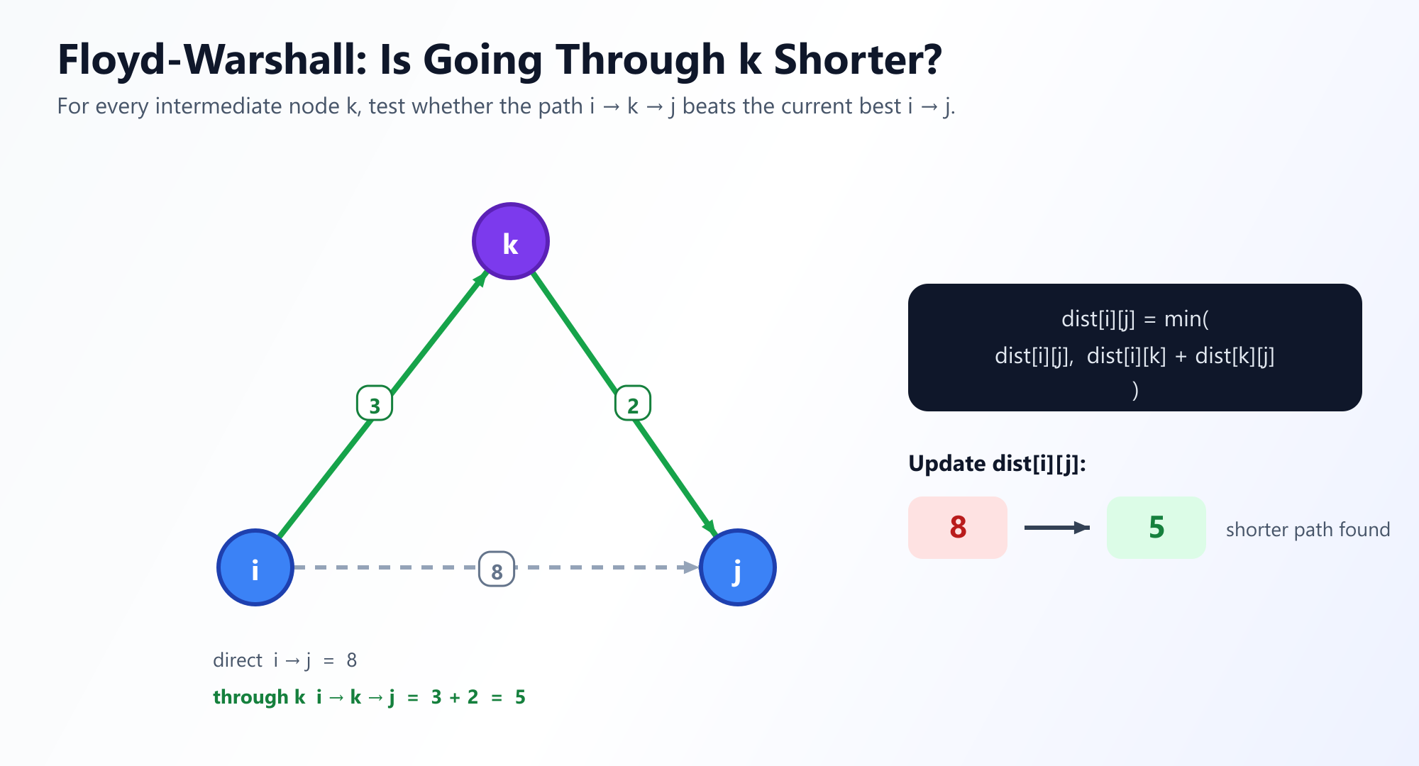
Suppose you already know every value of dk-1 and want dk. Consider the shortest path from i to j that may use {1, ..., k}. There are exactly two possibilities, and they are mutually exclusive:

1. The path does not use vertex k. Then it only uses {1, ..., k-1}, so its length is dk-1(i, j), a value you already have.
2. The path does use vertex k. Because a shortest path never repeats a vertex, it passes through k exactly once. That splits it into a leg from i to k and a leg from k to j, and neither leg may use k as an intermediate stop. So its length is dk-1(i, k) + dk-1(k, j), and both terms are also already known.

The shortest path is whichever of the two is smaller, which gives the recurrence at the heart of the algorithm:

d[k][i][j] = min( d[k-1][i][j],
                  d[k-1][i][k] + d[k-1][k][j] )

In words: routing through k is worth it only if the detour to k and onward to j is shorter than the best route found without it. This is dynamic programming in its purest form. Each subproblem is solved once, stored, and reused.

In practice nobody stores V separate matrices. The values can be updated in place in a single V x V matrix, because during iteration k the entries d(i, k) and d(k, j) cannot change: updating either would require d(k, k), which is 0 as long as the graph has no negative cycle. Reading a value that has already been overwritten in the same round is therefore harmless, and the space requirement drops from O(V3) to O(V2).

5. Step-by-Step Execution

Abstract recurrences become clear once they are run on numbers. Take a directed graph on four vertices with these edges:

• 1 -> 2 with weight 5
• 1 -> 4 with weight 10
• 2 -> 3 with weight 3
• 3 -> 4 with weight 1

Initialise the matrix from the edges alone. The diagonal is 0, because every vertex reaches itself at no cost, and every missing edge is infinity.

k = 0 (direct edges only)

        1     2     3     4
  1     0     5     inf   10
  2     inf   0     3     inf
  3     inf   inf   0     1
  4     inf   inf   inf   0

Round k = 1. Vertex 1 is now permitted as an intermediate stop. Any update would need a finite d(i, 1), but column 1 is infinite everywhere except the diagonal, because no edge leads into vertex 1. Nothing changes.

Round k = 2. Vertex 2 becomes available. Row 2 offers a finite d(2, 3) = 3, and column 2 offers a finite d(1, 2) = 5. That yields one candidate improvement:

• d(1, 3) was infinity. Through vertex 2 it becomes 5 + 3 = 8. Updated to 8.

Round k = 3. Vertex 3 becomes available, and d(3, 4) = 1. Two entries improve:

• d(1, 4) was 10 via the direct edge. Through vertex 3 it becomes d(1, 3) + d(3, 4) = 8 + 1 = 9. Updated to 9.
• d(2, 4) was infinity. Through vertex 3 it becomes 3 + 1 = 4. Updated to 4.

Notice that the improvement to d(1, 4) relied on d(1, 3) = 8, a value discovered in the previous round. The algorithm is building longer paths out of shorter ones it has already proved correct.

Round k = 4. Vertex 4 has no outgoing edges, so row 4 is infinite apart from the diagonal and no path can usefully pass through it. Nothing changes, and the algorithm terminates.

Final (all pairs)

        1     2     3     4
  1     0     5     8     9
  2     inf   0     3     4
  3     inf   inf   0     1
  4     inf   inf   inf   0

The answer for 1 -> 4 is 9, taking the route 1 -> 2 -> 3 -> 4 at a cost of 5 + 3 + 1, which beats the direct edge of weight 10. The remaining infinities are correct rather than unfinished: no edge enters vertex 1, so nothing can reach it.

6. Implementation and Pseudocode

The algorithm is short enough to memorise. The one detail that matters more than any other is the loop order.

function FloydWarshall(W, V):
    // W[i][j] = weight of edge i -> j, or Infinity if absent
    // dist is a V x V matrix

    for i from 1 to V:
        for j from 1 to V:
            dist[i][j] = W[i][j]
        dist[i][i] = 0

    // k MUST be the outermost loop
    for k from 1 to V:
        for i from 1 to V:
            for j from 1 to V:
                if dist[i][k] + dist[k][j] < dist[i][j]:
                    dist[i][j] = dist[i][k] + dist[k][j]

    return dist

k must be the outermost loop. This is the single most common way the algorithm is written incorrectly. The recurrence requires that every pair (i, j) be updated with respect to intermediate vertex k before moving on to k + 1. If k is placed innermost, the matrix is filled in an order that has no meaning, and the result is a set of distances that look plausible but are not optimal.

One implementation caution: if you represent infinity with a large sentinel integer such as INT_MAX rather than a true floating point infinity, then dist[i][k] + dist[k][j] can overflow and wrap around to a negative number, which the comparison will then happily accept. Either use a real infinity, or guard the addition by skipping the update when either operand is the sentinel.

7. Time and Space Complexity

• Time: O(V3). Three nested loops each run V times, and the body is a single comparison and assignment. There is no best case or worst case worth distinguishing: the algorithm performs exactly V3 relaxation tests on every input, regardless of how many edges the graph actually has.
• Space: O(V2). One distance matrix, updated in place. A second matrix of the same size is needed if you also want to reconstruct paths.

The insensitivity to E is the defining trait. A graph with four vertices and three edges costs the same as a graph with four vertices and twelve. That is wasteful on sparse graphs and perfectly efficient on dense ones. In exchange, the constant factor is very small and the memory access pattern is regular and cache friendly, so Floyd-Warshall often outruns its asymptotics on graphs of a few hundred vertices.

8. Negative Edges and Negative Cycle Detection

Floyd-Warshall accepts negative edge weights without modification. The recurrence never assumes that adding an edge increases a path's length, and that assumption is precisely what makes Dijkstra's algorithm fail on negative input.

Negative cycles are a different matter, and no algorithm can return meaningful shortest distances in their presence: you can lap the cycle indefinitely and drive the cost down without bound. What Floyd-Warshall gives you is a way to notice this for free. Inspect the diagonal after the algorithm finishes:

for i from 1 to V:
    if dist[i][i] < 0:
        report "negative cycle detected"

The diagonal was initialised to 0. A vertex can only end up with a negative distance to itself if there is a closed walk starting and ending at that vertex whose total weight is below zero, which is exactly the definition of a negative cycle. Where Bellman-Ford needs a dedicated extra pass over all edges to make the same determination, Floyd-Warshall needs only a glance at V entries it has already computed.

Note the scope of the check. It flags any negative cycle that the corresponding vertex takes part in. If the diagonal is clean, every distance in the matrix is trustworthy. If it is not, the finite values elsewhere in the matrix should be treated as meaningless rather than merely imprecise.

9. Reconstructing the Actual Paths

The distance matrix records how far apart two vertices are, but not which route achieves it. Recovering the route requires one extra matrix, and the cheapest scheme stores, for each pair, the next vertex along the path.

Initialise next[i][j] = j whenever a direct edge exists, and leave it null otherwise. Then, whenever the main loop improves dist[i][j] by routing through k, inherit the first step of the new route:

if dist[i][k] + dist[k][j] < dist[i][j]:
    dist[i][j] = dist[i][k] + dist[k][j]
    next[i][j] = next[i][k]

The assignment is next[i][k], not k. The first move on the improved journey from i to j is the first move on the journey from i to k, which may well be some other vertex entirely. Reading the path back out is then a short walk: start at i, repeatedly follow next, and stop on reaching j. This costs O(V2) extra space and no meaningful extra time.

10. Variants and Real-World Applications

The three-loop structure generalises well beyond shortest paths, because the recurrence needs only an operation that combines two legs and an operation that chooses between alternatives.

Transitive Closure (Warshall's Algorithm)

Replace addition with logical AND and minimum with logical OR, and the same loops compute reachability: whether a path exists between each pair at all, ignoring cost. This is Warshall's original 1962 result, and it is why the combined algorithm carries both names. It appears in compiler dataflow analysis, dependency resolution and database query planning.

Widest Path and Bottleneck Problems

Replace addition with minimum and minimum with maximum, and the algorithm finds the route whose narrowest link is as wide as possible. This is the natural formulation for maximum bandwidth routing in a network and for capacity planning in logistics.

Network Routing and Latency Matrices

Network operators frequently need a full matrix of latencies or hop counts between every pair of nodes in a topology. Backbone topologies tend to be dense and modest in vertex count, which is exactly the regime Floyd-Warshall was made for.

Currency Arbitrage

Model currencies as vertices and exchange rates as edges. Taking the negative logarithm of each rate turns multiplication of rates into addition of weights, and a profitable arbitrage loop turns into a negative cycle. The diagonal check then reports whether an arbitrage opportunity exists, and the next matrix reconstructs the sequence of trades.

11. Academic Resources and History

The algorithm has an unusually tangled attribution. Several researchers arrived at the same three loops independently within a few years of one another.

• Stephen Kleene (1956) described the underlying procedure while converting finite automata into regular expressions, which is structurally the same closure computation.
• Bernard Roy (1959) published the algorithm in essentially its modern form in Transitivite et connexite, three years before the papers that gave it its common name.
• Stephen Warshall (1962) published the transitive closure version, proving the Boolean matrix theorem that bears his name.
• Robert W. Floyd (1962) published the shortest path version as a remarkably brief note, Algorithm 97: Shortest Path, in Communications of the ACM.
• Peter Ingerman (1962) described the now standard three nested loop formulation in the same journal later that year.

For a rigorous treatment with full proofs of correctness, the standard reference is Cormen, Leiserson, Rivest and Stein, Introduction to Algorithms, in the chapter on all-pairs shortest paths. Readers comparing approaches for sparse graphs should also study Johnson's algorithm, which reweights a graph so that repeated Dijkstra remains valid even when negative edges are present. Full citations are listed at the end of this article.