Prim's MST Algorithm Explained

Mohammed Islam Hadjoudj

Expert Operations Research Engineer

1. Introduction to Prim's Algorithm

Prim's algorithm builds a minimum spanning tree: given a connected, undirected, weighted graph, it selects a subset of edges that touches every vertex, contains no cycle, and has the smallest possible total weight. For a graph with V vertices, that subset always contains exactly V - 1 edges.

The strategy is to grow a single tree outward. Start from any vertex, then repeatedly reach across the boundary of what you have built and pull in the cheapest edge that touches a vertex you do not yet own. Repeat V - 1 times and the tree is finished. There is no backtracking and nothing is ever removed.

That description sounds almost too greedy to be correct. Choosing the cheapest edge available right now, with no lookahead, is exactly the strategy that fails for shortest paths as soon as a negative edge appears. For minimum spanning trees it does not fail, and the reason is a single theorem worth understanding before touching any code.

2. Why It Works: The Cut Property

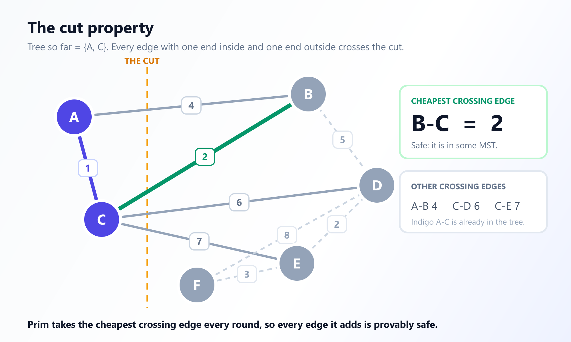
A cut splits the vertices into two non-empty groups. An edge crosses the cut if its two endpoints land in different groups. The theorem that underwrites Prim's algorithm is this:

The proof is short and worth seeing, because it explains the whole algorithm. Let e be the cheapest edge crossing some cut, and suppose a minimum spanning tree T does not contain it. Adding e to T creates exactly one cycle, and that cycle must cross the cut a second time, using some other edge f. Remove f. You still have a spanning tree, and since e was the cheapest crossing edge, its weight is no greater than that of f, so the new tree is no heavier. A minimum spanning tree therefore exists that contains e.

Now look at what Prim's algorithm does at every step. The vertices already in the tree form one side of a cut, and everything else forms the other. The algorithm selects the cheapest edge crossing precisely that cut. By the cut property, every edge it selects is safe: it belongs to some minimum spanning tree. The greedy choice is never a gamble that happens to pay off, it is a theorem applied V - 1 times.

3. How the Tree Grows

Concretely, the algorithm maintains three things: the set of vertices already in the tree, a key value for every vertex outside it, and a parent pointer recording which tree vertex offered that key.

• key[v] is the weight of the cheapest single edge connecting v to the current tree, or infinity if no such edge exists yet.
• parent[v] is the tree vertex at the other end of that edge. It is what lets you output the actual tree at the end rather than just its weight.

Each round takes the vertex outside the tree with the smallest key, adds it along with the edge to its parent, and then relaxes: for every neighbour w still outside the tree, if the edge to w is cheaper than key[w], lower key[w] and repoint parent[w].

Note carefully what the key represents. It is the weight of one edge, not the cost of a path. That single detail is what separates this algorithm from Dijkstra's, a point worth returning to once the code is on the page.

4. Step-by-Step Execution

Take the six-vertex graph used throughout our minimum spanning trees guide. Its nine edges are:

A-B 4    A-C 1    B-C 2
B-D 5    C-D 6    C-E 7
D-E 2    D-F 8    E-F 3

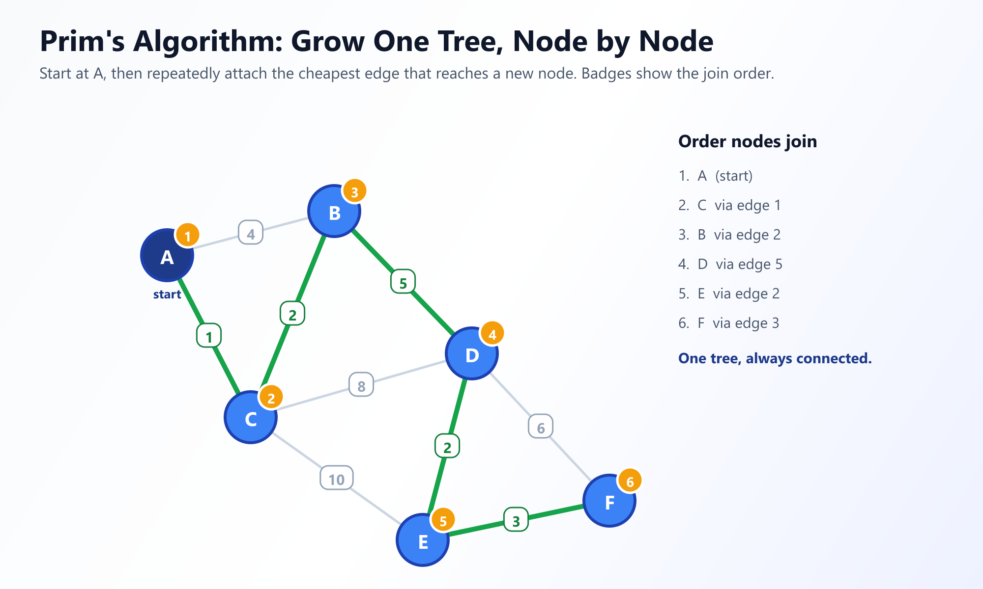
Start at A. At each round the "frontier" is the set of edges with exactly one endpoint inside the tree, and the algorithm takes the cheapest of them.

1. Tree = {A}. Frontier: A-C (1), A-B (4). Cheapest is A-C (1). Add C.
2. Tree = {A, C}. Frontier: B-C (2), A-B (4), C-D (6), C-E (7). Note that B is now reachable two ways, at 4 through A and at 2 through C, so its key drops to 2. Cheapest is B-C (2). Add B.
3. Tree = {A, C, B}. Frontier: B-D (5), C-D (6), C-E (7). D is reachable at 5 or 6, so its key is 5. Cheapest is B-D (5). Add D.
4. Tree = {A, C, B, D}. Frontier: D-E (2), C-E (7), D-F (8). E's key drops from 7 to 2. Cheapest is D-E (2). Add E.
5. Tree = {A, C, B, D, E}. Frontier: E-F (3), D-F (8). F's key drops from 8 to 3. Cheapest is E-F (3). Add F.

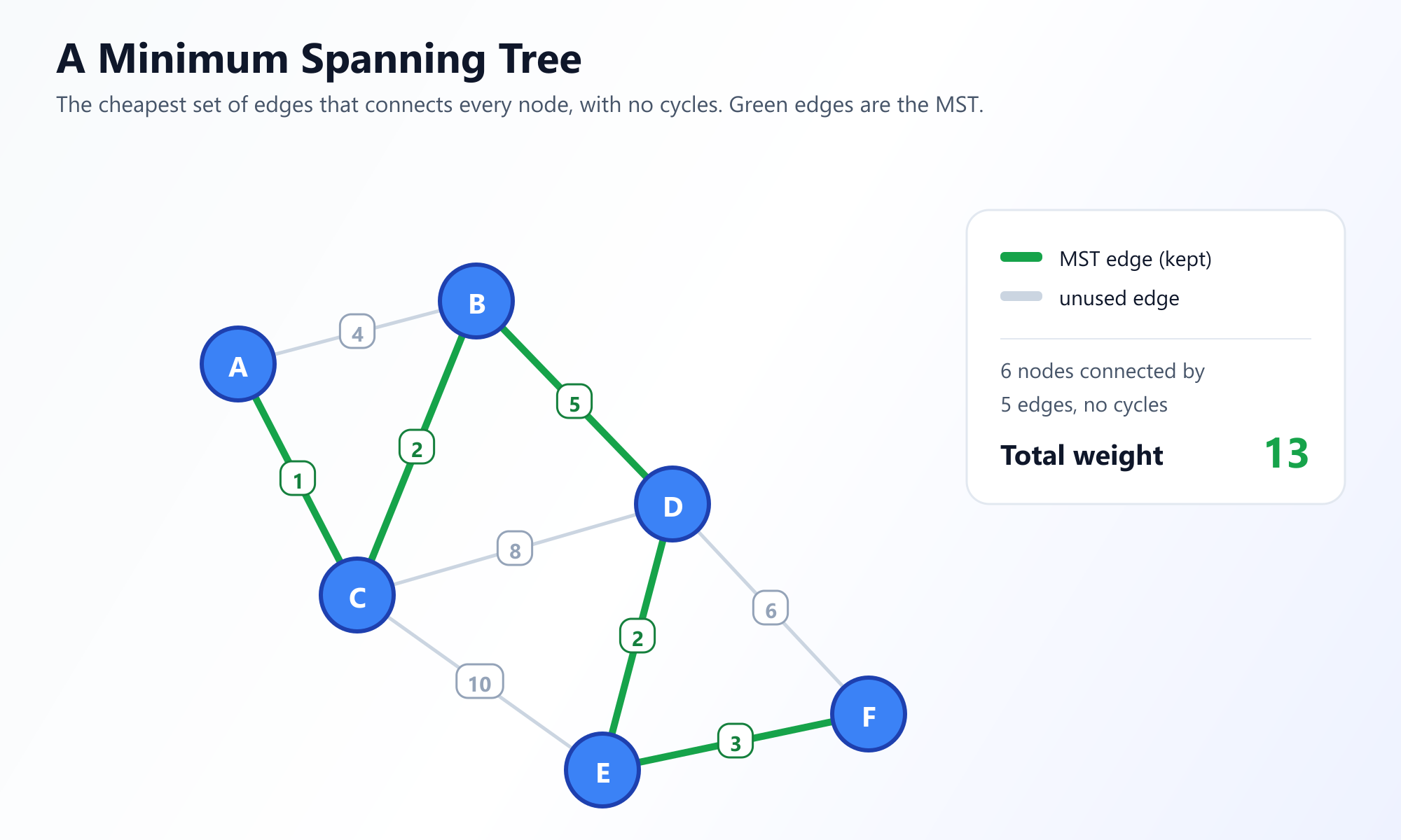
Five edges added for six vertices, and the algorithm stops. The tree is A-C (1), B-C (2), B-D (5), D-E (2), E-F (3), with a total weight of 13. The edges A-B (4), C-D (6), C-E (7) and D-F (8) are never used.

Two moments in that trace are worth dwelling on. In round 3 the algorithm accepted an edge of weight 5 while an edge of weight 2 (D-E) sat elsewhere in the graph untouched. Prim's cannot take D-E yet because neither endpoint is in the tree, and taking it would leave two disconnected fragments rather than one growing tree. In round 4 the key for E fell from 7 to 2 the moment D joined. Keys only ever decrease, and that is what makes the priority queue implementation efficient.

5. Implementation: Lazy and Eager Prim

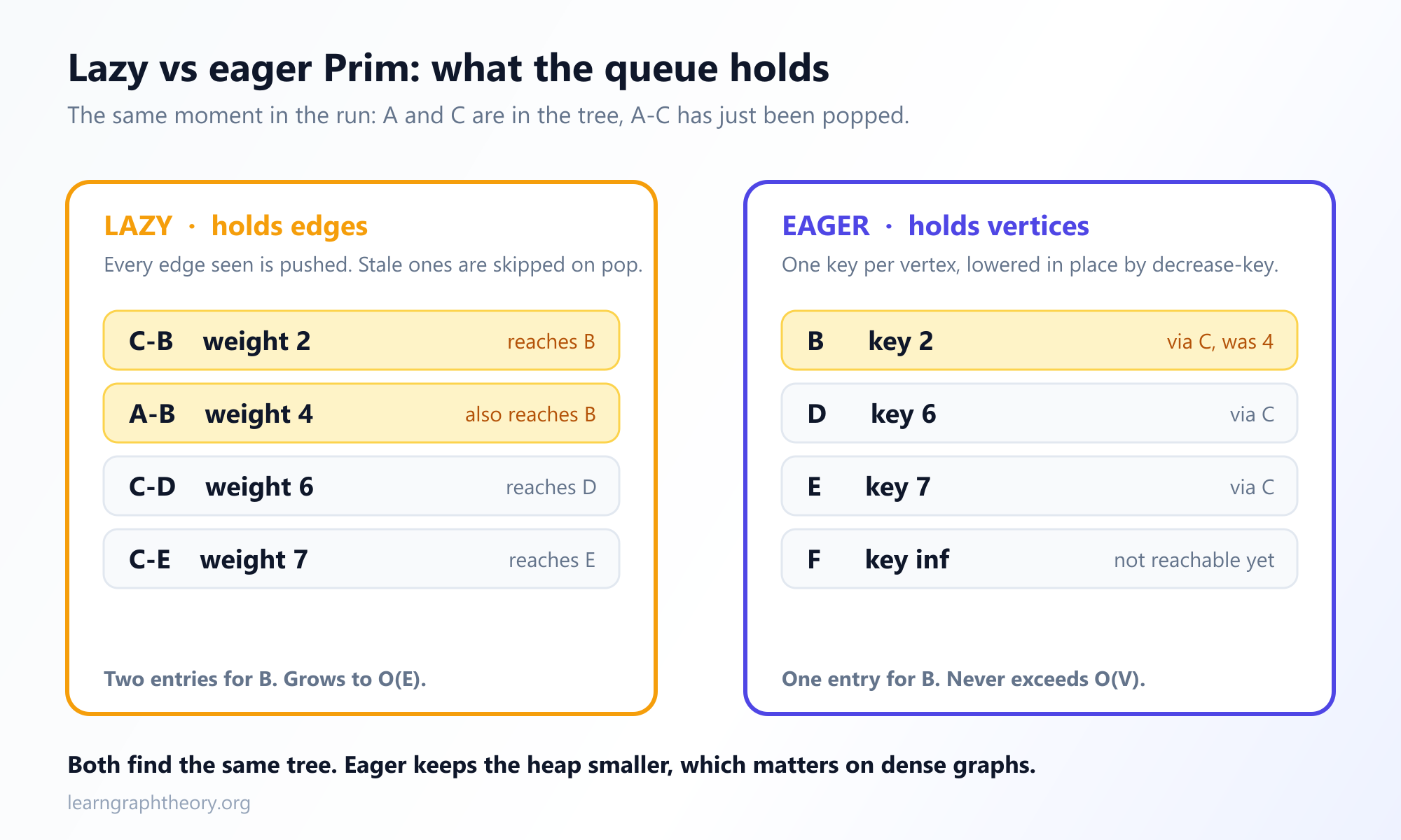
Two implementations are common, and the difference is what the priority queue holds.

Lazy Prim

The simpler version pushes every edge it encounters into a min-heap and discards entries that turn out to be stale when popped.

function LazyPrim(Graph, start):
    inTree = set()
    pq = empty min-heap keyed by edge weight
    mst = []

    visit(start)                    // mark it and push its edges

    while pq is not empty and size(mst) < V - 1:
        (w, u, v) = pq.pop()        // cheapest edge seen so far
        if v in inTree: continue    // stale: both ends already in the tree
        mst.append((u, v, w))
        visit(v)

    return mst

function visit(x):
    inTree.add(x)
    for each edge (x, y) with weight w:
        if y not in inTree: pq.push((w, x, y))

The if v in inTree: continue line is doing the real work. It is what prevents a cycle, and it is why the heap can safely hold obsolete entries: they are simply skipped when they surface.

Eager Prim

The eager version keeps at most one entry per vertex, the current key[v], and lowers it in place with a decrease-key operation. It needs an indexed priority queue, which is more machinery, but the heap never grows beyond V entries instead of E.

function EagerPrim(Graph, start):
    for each vertex v:
        key[v] = Infinity
        parent[v] = Null
    key[start] = 0
    pq = indexed min-heap of all vertices, keyed by key[]

    while pq is not empty:
        u = pq.popMin()
        inTree.add(u)
        for each edge (u, v) with weight w:
            if v not in inTree and w < key[v]:
                key[v] = w                  // the EDGE weight, not a sum
                parent[v] = u
                pq.decreaseKey(v, w)

    return parent            // parent[] is the tree

Prefer eager Prim on dense graphs, where E is far larger than V and holding every edge in the heap becomes wasteful. Lazy Prim is perfectly reasonable on sparse graphs and is considerably easier to get right.

6. Time and Space Complexity

• Lazy Prim, binary heap: O(E log E) time. Every edge may be pushed and popped once. Since E < V2, log E is O(log V), so this is usually written O(E log V). Space is O(E).
• Eager Prim, indexed binary heap: O(E log V) time, from V pop operations and up to E decrease-key operations, each O(log V). Space is O(V).
• Eager Prim, no heap, adjacency matrix: O(V2) time by scanning for the minimum key linearly. On a dense graph, where E approaches V2, this beats the heap version, because O(V2) is better than O(V2 log V).
• Eager Prim, Fibonacci heap: O(E + V log V), the best known bound for Prim's, since decrease-key becomes amortised constant time. The constant factors are large enough that it rarely wins in practice.

The practical summary: reach for a binary heap on sparse graphs and the plain O(V2) matrix scan on dense ones. The Fibonacci heap is mostly of theoretical interest.

7. Prim's vs Dijkstra's: One Line Apart

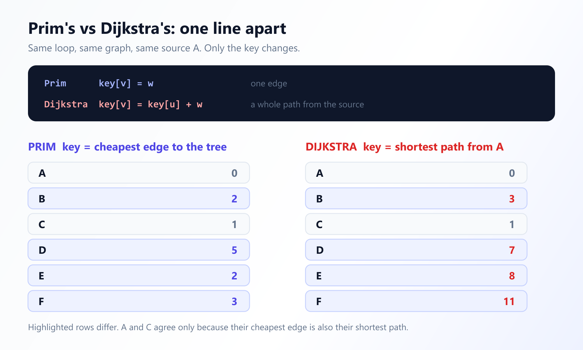
Set the eager Prim pseudocode beside Dijkstra's algorithm and they are nearly the same program. Both keep a key per vertex, both repeatedly extract the minimum, both relax the neighbours of whatever they just extracted. The entire difference is what goes into the key:

Prim:      if w < key[v]:              key[v] = w
Dijkstra:  if key[u] + w < key[v]:     key[v] = key[u] + w

Prim's key is the weight of a single edge. Dijkstra's key is the accumulated length of a whole path from the source. That is why they answer different questions: Prim's asks "what is the cheapest way to attach this vertex to my tree", and Dijkstra's asks "what is the cheapest way to reach this vertex from the source".

It also explains why negative weights break one and not the other. Dijkstra's correctness depends on path costs never decreasing as paths get longer, which a negative edge destroys. Prim's never adds weights together at all, so negative edge weights are completely harmless to it. A minimum spanning tree is well defined on a graph with negative weights, and Prim's finds it without modification.

8. Prim's vs Kruskal's

Both algorithms are greedy, both are justified by the cut property, and on a graph with distinct weights both return the identical tree. They differ in what they keep connected along the way.

• Prim's maintains one connected tree at all times and grows it outward. It never sorts the edges, and it needs a priority queue.
• Kruskal's sorts all edges by weight and adds each one unless it would close a cycle, so it maintains a forest of fragments that only merge into one tree at the very end. It needs a union-find structure.

The practical rule follows from density. Kruskal's cost is dominated by sorting, at O(E log E), which is excellent when E is small. Prim's with an adjacency matrix runs in O(V2) regardless of edge count, which wins when the graph is dense. There is also a structural difference on disconnected input: Kruskal's naturally produces a minimum spanning forest, while Prim's from a single start vertex only ever spans that vertex's component, so you must restart it once per component.

9. Practical Notes and Common Pitfalls

Four situations trip people up when they move from the textbook version to real input.

• Tied weights mean several valid answers. When two edges share a weight, the graph can have more than one minimum spanning tree, and which one you get depends on how your priority queue breaks ties. All of them are equally optimal, so a test that compares against one hard-coded edge list will fail spuriously. Compare total weight instead.
• Disconnected input fails quietly. Started from one vertex, Prim's spans only that vertex's component and then stops, returning a tree that looks perfectly valid. The check is to count: a genuine spanning tree has exactly V - 1 edges. Fewer means the graph was disconnected, and you need to restart from an unvisited vertex to collect the remaining components.
• Self-loops and parallel edges. A self-loop can never cross a cut, so it is always ignorable. Among parallel edges between the same pair of vertices, only the cheapest can ever be chosen. Neither breaks the algorithm, but filtering them during input parsing keeps the heap smaller.
• Directed graphs are a different problem entirely. A minimum spanning tree is defined for undirected graphs. Feeding directed edges to Prim's produces something that is not meaningful. The directed analogue is a minimum spanning arborescence, found by Edmonds' algorithm, and it is materially harder.

10. Real-World Applications

Minimum spanning trees answer one recurring question: what is the cheapest way to connect everything, with no redundancy? Prim's suits the cases where the network genuinely grows from a source.

Utility and Network Layout

Laying cable, fibre, water pipe or road between a fixed set of sites, where every site must be reachable and total length or cost is what you are minimising, is the original motivation. Prim's paper came out of exactly this problem at Bell Labs.

Cluster Analysis

Building the minimum spanning tree of a point set and then deleting its heaviest edges is single-linkage clustering: removing the k - 1 heaviest edges leaves exactly k clusters. The tree is computed once and every value of k falls out of it.

Approximation for Harder Problems

The minimum spanning tree gives a lower bound on the travelling salesman tour, and doubling its edges yields a tour at most twice optimal on metric instances. It is the starting point for the Christofides construction, which improves that guarantee to 1.5.

Image Segmentation and Maze Generation

Treat pixels as vertices and dissimilarity as edge weight, and MST-based segmentation groups a picture into regions. Run Prim's on a grid with random weights instead and you get a uniform-looking maze, which is why it is a staple of procedural generation.

11. Academic Resources and History

Like several classical graph algorithms, this one was discovered more than once, and the name it carries is not the name of the person who found it first.

• Otakar Borůvka (1926) posed and solved the minimum spanning tree problem first, motivated by electrifying rural Moravia. His algorithm is a different one, adding the cheapest edge out of every fragment in parallel rounds.
• Vojtěch Jarník (1930) published the algorithm we now call Prim's, in a letter responding to Borůvka. This is why the algorithm is sometimes correctly called the Jarník-Prim algorithm.
• Robert C. Prim (1957) rediscovered it independently at Bell Laboratories while studying the cost of connection networks, and his paper is the one that reached a wide audience.
• Edsger W. Dijkstra (1959) rediscovered it a third time, in the same short paper that introduced his shortest path algorithm, which is no coincidence given how close the two are.

For the definitive account of who found what and when, see Graham and Hell's history of the problem. For a rigorous treatment with full proofs of the cut property and both algorithms, the standard reference is Cormen, Leiserson, Rivest and Stein, Introduction to Algorithms, in the chapter on minimum spanning trees. Readers interested in how far the complexity has been pushed should look at Fredman and Tarjan's Fibonacci heap result and Chazelle's near-linear algorithm. Full citations appear at the end of this article.