
Table of Contents
- 1. What makes a graph planar
- 2. Faces: the regions a drawing creates
- 3. Euler's formula
- 4. How many edges can a planar graph have?
- 5. Why K₅ and K₃,₃ are not planar
- 6. Kuratowski's and Wagner's theorems
- 7. Testing planarity
- 8. Colouring planar graphs and the four colour theorem
- 9. Dual graphs
- 10. Where planar graphs show up
- 11. Beyond the plane: crossings and surfaces
- 12. Common mistakes
- 13. Glossary
- 14. Frequently asked questions
- 15. References
1. What makes a graph planar
A graph is planar when it can be drawn on a flat sheet of paper so that no two edges cross. Each vertex becomes a point, each edge becomes a curve joining its two end points, and curves are allowed to meet only at a vertex they share. A drawing that obeys these rules is called a plane drawing or an embedding of the graph, and a graph together with one fixed embedding is a plane graph.
The distinction between the two words matters more than it first seems. Planar is a property of the graph: it asks whether some crossing-free drawing exists. Plane describes one particular drawing. A graph can have a perfectly good plane drawing and also a hundred drawings full of crossings, and none of the bad drawings counts against it. The complete graph K4 is the standard first example. Drawn as a square with both diagonals, its two diagonals cross. Move one vertex into the middle of the triangle formed by the other three and every crossing disappears, so K4 is planar.
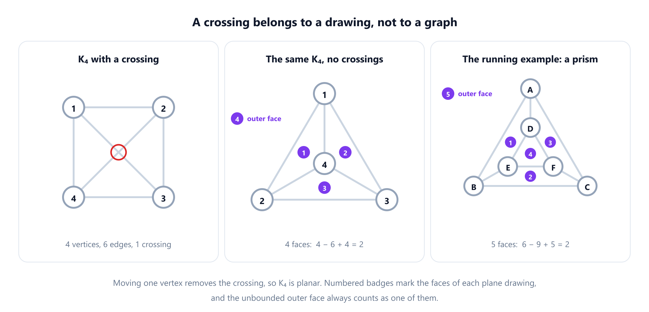
The figure also introduces the running example for this article, the triangular prism. It has an outer triangle A, B, C, an inner triangle D, E, F, and three spokes joining A to D, B to E and C to F:
V = {A, B, C, D, E, F}                                   6 vertices
E = {AB, BC, CA, DE, EF, FD, AD, BE, CF}                  9 edges
Three practical remarks settle what the definition does and does not depend on. First, loops and parallel edges never affect planarity: a second copy of an edge can be drawn as a thin curve right next to the first, and a loop as a small curl beside its vertex. A multigraph is planar exactly when its underlying simple graph is, which is why the counting bounds later in this article are stated for simple graphs. Second, the plane and the sphere are interchangeable. Stereographic projection turns a drawing on a sphere into a drawing in the plane and back again, so a graph is planar exactly when it can be drawn on the surface of a ball without crossings. Third, curves are never needed. Wagner in 1936 and Fáry in 1948 proved independently that every simple planar graph has a plane drawing in which every edge is a straight line segment, a result usually called Fáry's theorem.
2. Faces: the regions a drawing creates
Cut a plane drawing out of the paper along its edges and the paper falls apart into pieces. Those pieces are the faces of the drawing. Exactly one of them is unbounded; it is called the outer face, and forgetting to count it is the most common slip in this whole subject. The triangular prism has five faces: the inner triangle D, E, F, three four-sided faces A, B, E, D, B, C, F, E and C, A, D, F, and the outer face, which lies outside the triangle A, B, C.
The length (or degree) of a face is the number of edges you walk along when you trace its boundary, with one rule that keeps the bookkeeping exact: an edge that has the same face on both of its sides, such as an edge of a tree, is walked twice and counted twice. With that rule every edge contributes exactly two to the total, one for each of its sides, and the faces obey a handshaking lemma of their own:
sum of the face lengths = 2e

prism:   3 + 4 + 4 + 4 + 3  =  18  =  2 × 9
         (inner triangle, three quadrilaterals, outer face bounded by A, B, C)
This identity is the vertex handshaking lemma from the vertices and edges guide with faces in place of vertices, and it powers every bound in sections 4 and 5. Faces belong to a drawing rather than to the graph, so a graph with several plane drawings can have faces of different lengths in each. Join two vertices x and y by four paths of lengths 1, 2, 3 and 4. Arranged around x in that order, consecutive paths bound faces of lengths 3, 5, 7 and 5. Swap the middle two paths and the face lengths become 4, 5, 6 and 5. What does not change is the number of faces, four in both drawings, and the next section proves that this is no accident.
3. Euler's formula
Count the vertices, edges and faces of any connected plane drawing and one combination of the three never changes.
Euler's formula. For every connected plane graph withvvertices,eedges andffaces,v − e + f = 2.
For the prism, 6 − 9 + 5 = 2. For K4 drawn without crossings, 4 − 6 + 4 = 2. For a single vertex, 1 − 0 + 1 = 2, since the empty plane around it is one face. The proof is short enough to give in full, and it is worth reading because the same idea, deleting an edge and watching what changes, runs through the rest of the subject.
Proof. Fix the number of vertices and use induction on the number of edges. A connected graph with as few edges as possible is a tree, and a tree has e = v − 1 (one of the characterisations collected in trees in graph theory). A tree contains no cycle, so its drawing does not enclose any region and there is just one face. Then v − (v − 1) + 1 = 2, as claimed.
If the connected graph is not a tree, it contains a cycle. Pick an edge on that cycle and delete it. The graph stays connected, because the rest of the cycle still links the two ends of the deleted edge. In the drawing, the cycle is a closed curve, and by the Jordan curve theorem it separates the plane into an inside and an outside. The deleted edge therefore had different faces on its two sides, one inside the cycle and one outside, and removing it merges those two faces into one. So e drops by one and f drops by one, and v − e + f is unchanged. By the induction hypothesis the smaller graph satisfies the formula, so the original graph does too.
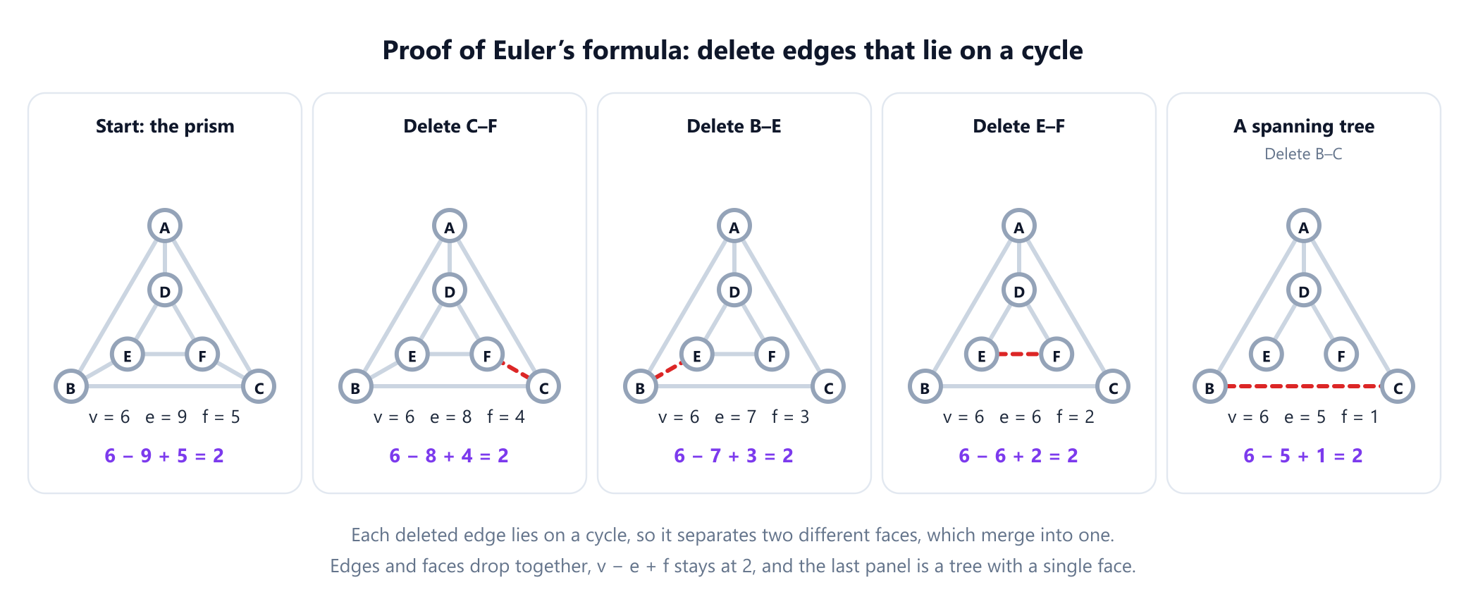
The formula has a consequence that is easy to read past. The number of faces, f = e − v + 2, depends only on the graph and not on how it is drawn. That is why the two drawings of the four-path graph in section 2 both had four faces: with v = 8 and e = 10, every plane drawing of that graph has 10 − 8 + 2 = 4 faces. If the graph is not connected the outer face is shared by all the pieces, and the formula becomes v − e + f = 1 + k for a graph with k components.
The formula is easy to check by machine. The function below takes a crossing-free straight-line drawing, given as coordinates, and traces every face by walking along the edges and always turning to the next edge in clockwise order at each vertex. Each edge has two sides, and each side is walked exactly once.
from math import atan2

def faces(pos, edges):
    """Trace the faces of a crossing-free straight-line drawing of a connected graph."""
    nbrs = {v: [] for v in pos}
    for u, v in edges:
        nbrs[u].append(v)
        nbrs[v].append(u)
    for v, ws in nbrs.items():               # neighbours in anticlockwise order
        x, y = pos[v]
        ws.sort(key=lambda w: atan2(pos[w][1] - y, pos[w][0] - x))
    seen, found = set(), []
    for u, v in edges:
        for dart in ((u, v), (v, u)):        # each edge has two sides
            face = []
            while dart not in seen:
                seen.add(dart)
                a, b = dart
                face.append(a)
                ws = nbrs[b]
                dart = (b, ws[ws.index(a) - 1])  # at b, turn to the next edge clockwise
            if face:
                found.append(face)
    return found

pos = {'A': (0, 4), 'B': (-3.5, -2), 'C': (3.5, -2),
       'D': (0, 1.6), 'E': (-1.4, -0.8), 'F': (1.4, -0.8)}
edges = [('A', 'B'), ('B', 'C'), ('C', 'A'), ('D', 'E'), ('E', 'F'),
         ('F', 'D'), ('A', 'D'), ('B', 'E'), ('C', 'F')]
fs = faces(pos, edges)
v, e, f = len(pos), len(edges), len(fs)
print(v, e, f, v - e + f)
# 6 9 5 2
print(sorted(len(face) for face in fs))
# [3, 3, 4, 4, 4]
The five face lengths are exactly the ones counted in section 2, and their sum is 18 = 2e. The same tracing procedure, run on an abstract list of neighbour orders rather than on coordinates, is how planarity libraries store an embedding: an embedding of a graph is fully described by the cyclic order of the edges around every vertex, a description known as a rotation system.
Polyhedra, and where the formula came from
Euler did not state the formula for graphs. He stated it for polyhedra, solids bounded by flat faces, in a letter to Christian Goldbach in November 1750, and published it in two papers in the St Petersburg Academy's journal, in the volume dated 1752 and 1753 that was printed in 1758. Draw a convex polyhedron in the plane by looking through one of its faces, which then becomes the outer face, and its corners, edges and faces become the vertices, edges and faces of a plane graph. The five Platonic solids all give the same answer:
| Solid | v | e | f | v − e + f |
|---|---|---|---|---|
| Tetrahedron | 4 | 6 | 4 | 2 |
| Cube | 8 | 12 | 6 | 2 |
| Octahedron | 6 | 12 | 8 | 2 |
| Dodecahedron | 20 | 30 | 12 | 2 |
| Icosahedron | 12 | 30 | 20 | 2 |
The history has two well-known twists. René Descartes had written down an equivalent relation, phrased in terms of angles, in a manuscript that is now lost; a copy that Leibniz made in Paris in 1675 or 1676 was rediscovered in the nineteenth century and published in 1859–60. And Euler's own argument, which sliced corners off the solid one at a time, was not a complete proof by modern standards. Adrien-Marie Legendre gave the first complete proof in 1794, using the areas of polygons drawn on a sphere, and Augustin-Louis Cauchy published another in 1813 that flattens the polyhedron into a network in the plane and takes it apart piece by piece, close in spirit to the argument above. Imre Lakatos built his book Proofs and Refutations (1976) around the strange "polyhedra" that break the formula, such as a picture frame, whose surface has a hole. The history of graph theory places this result next to Euler's other founding contribution, the bridges of Königsberg.
4. How many edges can a planar graph have?
Euler's formula turns into a hard limit on the number of edges once it is combined with the face handshaking lemma. The argument is the most useful three lines in the theory of planar graphs.
Theorem. A simple planar graph withv ≥ 3vertices has at most3v − 6edges. If it also has no triangles, it has at most2v − 4edges.
Proof. Take a plane drawing and assume first that the graph is connected. In a simple graph with at least three vertices, every face has length at least 3: a face of length 1 would need a loop and a face of length 2 would need two parallel edges, except when the whole graph is a single edge, which v ≥ 3 rules out. Adding up over all faces, 3f ≤ 2e. Euler's formula gives f = 2 − v + e, so 3(2 − v + e) ≤ 2e, which rearranges to e ≤ 3v − 6. If the graph has no triangles, every face has length at least 4, so 4f ≤ 2e and the same substitution gives e ≤ 2v − 4. A disconnected planar graph can have edges added between its components without creating any crossing, and adding edges only makes the inequality harder to satisfy, so the bounds hold for it as well.
The second bound covers every bipartite graph, since a bipartite graph has no odd cycles and in particular no triangles. Both bounds are special cases of one inequality. If the shortest cycle in a connected planar graph, its girth, has length g, every face has length at least g, and the same three lines give
e ≤ g(v − 2) / (g − 2)

g = 3   →   e ≤ 3v − 6        (any simple planar graph, v ≥ 3)
g = 4   →   e ≤ 2v − 4        (no triangles, so every bipartite planar graph)
g = 5   →   e ≤ 5(v − 2)/3     (no cycles of length 3 or 4)
The first bound is attained. A plane graph in which every face, including the outer one, is a triangle is called a triangulation, and for a triangulation 3f = 2e holds with equality, so e = 3v − 6 exactly. The octahedron (6 vertices, 12 edges) and the icosahedron (12 vertices, 30 edges) are triangulations. Adding any edge to a triangulation makes it non-planar, which is why triangulations are also called maximal planar graphs. The prism is not maximal: it has 9 edges against a ceiling of 3 × 6 − 6 = 12, and three diagonals, one in each quadrilateral face, would bring it up to 12.
Two corollaries are used constantly. The first is that planar graphs are sparse: the number of edges grows only linearly with the number of vertices, so a planar graph with a million vertices has fewer than three million edges, while a general graph on a million vertices may have almost 500 billion. That is why algorithms on planar graphs are measured against v alone, and why adjacency lists rather than matrices are the natural storage format, as discussed in graph representation. The second is the degree-five lemma:
Every simple planar graph has a vertex of degree at most 5.
The sum of the degrees is 2e, and 2e ≤ 6v − 12 when v ≥ 3, so the average degree is below 6 and some vertex must have degree 5 or less. Graphs with one or two vertices satisfy the lemma trivially. The lemma is sharp: every vertex of the icosahedron has degree exactly 5. It is the engine behind the colouring theorems in section 8.
5. Why K₅ and K₃,₃ are not planar
The edge bounds turn "no drawing works" from a claim about infinitely many drawings into a one-line calculation.
The complete graph K5 has v = 5 and e = 10. A planar graph on 5 vertices has at most 3 × 5 − 6 = 9 edges, so K5 is not planar.
The complete bipartite graph K3,3 has v = 6 and e = 9. The first bound allows 12 edges, so it says nothing. But K3,3 is bipartite and therefore has no triangles, and the second bound allows only 2 × 6 − 4 = 8. Nine edges are one too many. This is the classic three utilities puzzle, which asks you to connect three houses to water, gas and electricity without any pipes or cables crossing. It appears as "Water, Gas, and Electricity" in Henry Dudeney's Amusements in Mathematics of 1917, and the bipartite graphs guide gives the same argument from the bipartite side.
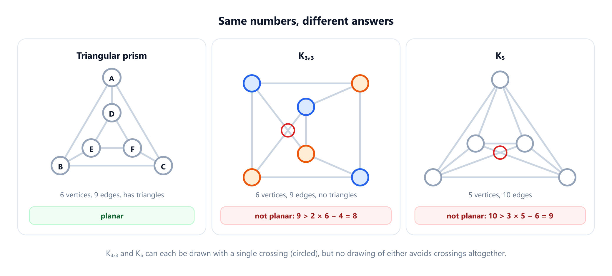
The comparison with the prism is the instructive part. Both graphs have six vertices and nine edges, and both have every vertex of degree 3, so no count of vertices, edges or degrees can tell them apart. What separates them is the shape of their faces: the prism can use two triangles, while K3,3 would need every face to have at least four sides, and there is not enough room for that.
Both graphs are only just non-planar. Each can be drawn with exactly one crossing, as the figure shows, so their crossing number is 1. Deleting any single edge from either graph leaves a planar graph. They are, in a precise sense, the smallest obstacles to planarity, and the next section explains that they are the only ones.
The counting bounds have a limit that has to be stated clearly: they are necessary conditions, not sufficient ones. A graph that violates them is certainly not planar; a graph that satisfies them may still be non-planar. Take K3,3 and add one edge between two vertices on the same side. The new graph has 6 vertices and 10 edges and now contains triangles, so the only bound that applies is 3v − 6 = 12, which it satisfies. Yet it contains K3,3, so it cannot be planar. The Petersen graph sits in between. With 10 vertices and 15 edges it passes both 3v − 6 = 24 and 2v − 4 = 16, but its girth is 5, and the girth bound allows only 5 × 8 / 3, about 13.3, so 13 edges. Fifteen edges are too many, and the Petersen graph is not planar.
6. Kuratowski's and Wagner's theorems
Two operations relate a graph to the small obstacles inside it. A subdivision of a graph replaces edges by paths, inserting new vertices of degree 2 along them. Subdividing an edge does not change whether a drawing has crossings, since the new vertices simply sit on the curve, so a subdivision of K5 or K3,3 is just as non-planar as the original. A planar graph also cannot contain a non-planar subgraph, because deleting parts of a plane drawing leaves a plane drawing. In 1930 Kazimierz Kuratowski proved that these obvious obstacles are the only ones.
Kuratowski's theorem (1930). A graph is planar if and only if it contains no subgraph that is a subdivision ofK5or ofK3,3.
The "only if" half is the easy direction just described. The "if" half is the deep one: any graph that cannot be drawn in the plane must contain one of these two shapes, possibly with its edges stretched into long paths. A second operation gives a cleaner version. Contracting an edge merges its two ends into one vertex adjacent to all their former neighbours, and a graph obtained from G by deleting vertices and edges and contracting edges is a minor of G. Contraction also preserves planarity, since you can shrink an edge of a plane drawing down to a point.
Wagner's theorem (1937). A graph is planar if and only if it has neitherK5norK3,3as a minor.
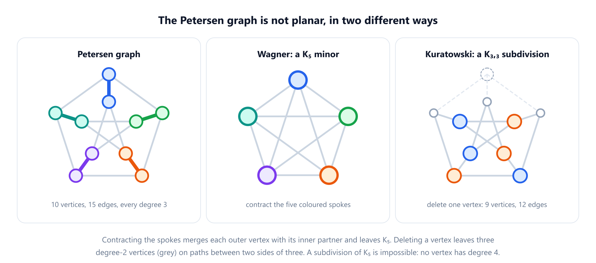
The two theorems are equivalent, but they are not interchangeable in examples, and the Petersen graph shows the difference. Contract the five spokes that join its outer 5-cycle to its inner pentagram and the ten vertices collapse to five, each adjacent to all four others: the Petersen graph has a K5 minor. It contains no subdivision of K5, though, because a subdivision of K5 needs five vertices of degree 4 and every vertex of the Petersen graph has degree 3. Kuratowski's theorem is still satisfied, by the other shape. Delete any one vertex and the remaining 9 vertices and 12 edges form a subdivision of K3,3: three of the vertices have degree 2 and sit on paths, and the other six split into two sides of three.
Wagner's form opened a much larger story. Planarity is minor-closed: every minor of a planar graph is planar. Neil Robertson and Paul Seymour proved, in a series of papers published between 1983 and 2004, that every minor-closed family of graphs is characterised by a finite list of forbidden minors, just as planar graphs are characterised by the list K5, K3,3. The theorem guarantees that such a list exists and is finite, but it does not say how long the list is or how to find it.
7. Testing planarity
The counting bounds from section 4 give an instant first test. They cannot prove that a graph is planar, but when they fail they prove that it is not, and they cost almost nothing to check. The function below computes the girth with a breadth-first search from every vertex and applies the girth bound, which includes both 3v − 6 and 2v − 4 as special cases.
from collections import deque

def girth(adj):
    """Length of the shortest cycle (inf for a forest): BFS from every vertex."""
    best = float('inf')
    for s in adj:
        dist, parent = {s: 0}, {s: None}
        queue = deque([s])
        while queue:
            u = queue.popleft()
            for w in adj[u]:
                if w not in dist:
                    dist[w], parent[w] = dist[u] + 1, u
                    queue.append(w)
                elif parent[u] != w:         # a non-tree edge closes a cycle
                    best = min(best, dist[u] + dist[w] + 1)
    return best

def euler_filter(adj):
    """False: certainly not planar. True: only 'not ruled out'. Simple, connected graphs."""
    n = len(adj)
    m = sum(len(ws) for ws in adj.values()) // 2
    g = girth(adj)
    if g == float('inf'):
        return True                          # trees are always planar
    return m * (g - 2) <= g * (n - 2)        # g = 3 gives 3n - 6, g = 4 gives 2n - 4

def graph(edges):
    adj = {}
    for u, v in edges:
        adj.setdefault(u, []).append(v)
        adj.setdefault(v, []).append(u)
    return adj

prism = graph(['AB', 'BC', 'CA', 'DE', 'EF', 'FD', 'AD', 'BE', 'CF'])
k5 = graph([(i, j) for i in range(5) for j in range(i + 1, 5)])
k33 = graph([(a, b) for a in 'abc' for b in 'xyz'])
petersen = graph([(i, (i + 1) % 5) for i in range(5)] + [(i, i + 5) for i in range(5)]
                 + [(5 + i, 5 + (i + 2) % 5) for i in range(5)])
k33_plus = graph([(a, b) for a in 'abc' for b in 'xyz'] + [('a', 'b')])
for name, adj in [('prism', prism), ('K5', k5), ('K3,3', k33),
                  ('Petersen', petersen), ('K3,3 + edge', k33_plus)]:
    print(f'{name:12} girth {girth(adj)}  passes: {euler_filter(adj)}')
# prism        girth 3  passes: True
# K5           girth 3  passes: False
# K3,3         girth 4  passes: False
# Petersen     girth 5  passes: False
# K3,3 + edge  girth 3  passes: True
The filter rejects K5, K3,3 and the Petersen graph, and it waves through the prism, which is correct, and K3,3 with an extra edge, which is not. "Passes" only ever means "not ruled out". Each breadth-first search takes O(v + e) time and the filter runs one from every vertex, so it costs O(v(v + e)); a graph that fails the cheaper test e ≤ 3v − 6 can be rejected before computing the girth at all.
A complete answer needs a real planarity algorithm. Kuratowski's theorem does not give an efficient one directly, since searching for subdivisions is expensive. Hopcroft and Tarjan published the first linear-time planarity test in 1974, building on depth-first search, and later algorithms made the idea simpler to implement: Boyer and Myrvold's edge-addition method of 2004, and the left-right planarity criterion of de Fraysseix and Rosenstiehl, on which the NetworkX implementation is based. A good implementation returns a certificate either way: a plane embedding when the graph is planar, and a Kuratowski subgraph when it is not.
import networkx as nx

def count_faces(embedding):
    seen, f = set(), 0
    for u, v in embedding.edges():           # every half-edge lies on exactly one face
        if (u, v) not in seen:
            embedding.traverse_face(u, v, mark_half_edges=seen)
            f += 1
    return f

tests = [('prism', nx.circular_ladder_graph(3)), ('K5', nx.complete_graph(5)),
         ('K3,3', nx.complete_bipartite_graph(3, 3)), ('Petersen', nx.petersen_graph()),
         ('K3,3 + edge', nx.complete_bipartite_graph(3, 3))]
tests[-1][1].add_edge(0, 1)
for name, G in tests:
    planar, cert = nx.check_planarity(G, counterexample=True)
    if planar:
        print(f'{name:12} planar, {count_faces(cert)} faces')
    else:
        branch = sum(1 for _, d in cert.degree() if d > 2)
        kind = 'K5' if branch == 5 else 'K3,3'
        print(f'{name:12} not planar: a subdivision of {kind}, '
              f'{cert.number_of_nodes()} vertices, {cert.number_of_edges()} edges')
# prism        planar, 5 faces
# K5           not planar: a subdivision of K5, 5 vertices, 10 edges
# K3,3         not planar: a subdivision of K3,3, 6 vertices, 9 edges
# Petersen     not planar: a subdivision of K3,3, 9 vertices, 12 edges
# K3,3 + edge  not planar: a subdivision of K3,3, 6 vertices, 9 edges
Every answer comes with its proof. For the prism the certificate is an embedding, stored as a rotation system, and tracing it gives 5 faces as Euler's formula requires. For K5 and K3,3 the certificate is the whole graph. For the Petersen graph it is a subdivision of K3,3 using 9 of the 10 vertices, exactly the structure in the right panel of the figure above, and it could never be a subdivision of K5 since no vertex has degree 4. Kuratowski subgraphs are not unique, so another library or version may return a different one; any of them is a valid proof.
8. Colouring planar graphs and the four colour theorem
Planar graphs have their most famous theorem in colouring. A proper colouring gives every vertex a colour so that the two ends of every edge differ, and the smallest number of colours that works is the chromatic number, covered in depth in the graph colouring guide. Colouring a map so that neighbouring countries differ is the same problem on the map's planar graph, with one vertex per country and an edge for every shared border.
The degree-five lemma from section 4 already gives a bound with an elementary proof.
Six colour theorem. Every planar graph can be properly coloured with at most six colours.
Remove a vertex of degree at most 5, which exists by the lemma, and colour the rest of the graph, which is still planar, by induction. Then put the vertex back. It has at most five neighbours, so at least one of six colours is free for it. The proof is an algorithm: repeatedly remove a vertex of smallest degree, then colour the vertices in reverse order of removal.
def six_colour(adj):
    """Colour a simple planar graph with at most 6 colours (smallest-last greedy)."""
    deg = {v: len(ws) for v, ws in adj.items()}
    removed, order = set(), []
    while len(order) < len(adj):
        v = min((u for u in adj if u not in removed), key=deg.get)  # degree <= 5 exists
        removed.add(v)
        order.append(v)
        for w in adj[v]:
            if w not in removed:
                deg[w] -= 1
    colour = {}
    for v in reversed(order):                # at most 5 neighbours are coloured already
        used = {colour[w] for w in adj[v] if w in colour}
        colour[v] = min(c for c in range(6) if c not in used)
    return colour

# The icosahedron: 12 vertices, 30 edges, every vertex of degree exactly 5.
edges = []
for i in range(5):
    j = (i + 1) % 5
    top, a, b, c, d, bottom = 0, 1 + i, 1 + j, 6 + i, 6 + j, 11
    edges += [(top, a), (a, b), (a, c), (a, d), (c, d), (c, bottom)]
adj = {v: [] for v in range(12)}
for u, v in edges:
    adj[u].append(v)
    adj[v].append(u)
colour = six_colour(adj)
print(len(edges), {len(ws) for ws in adj.values()}, max(colour.values()) + 1)
# 30 {5} 4
print(all(colour[u] != colour[v] for u, v in edges))
# True
On the icosahedron, where every vertex has degree exactly 5, the method uses four colours, which is the minimum, since each vertex and the five neighbours around it already need four. The ordering heuristic does not always do that well, but it never needs more than six.
Getting to five colours takes one more idea. In 1879 Alfred Kempe published a proof that four colours always suffice, based on swapping the two colours along a chain of alternately coloured vertices, now called a Kempe chain. In 1890 Percy Heawood found a flaw in Kempe's argument, and in the same paper rescued the chain technique to prove that five colours always suffice. The question itself goes back to 1852, when Francis Guthrie noticed that four colours were enough for a map of the counties of England and asked whether that was always true; his brother Frederick passed the question to Augustus De Morgan.
Four colour theorem (Appel and Haken, 1976). Every planar graph can be properly coloured with at most four colours.
Kenneth Appel and Wolfgang Haken announced the proof in 1976 and published it in 1977. It reduces the problem to a finite set of configurations, 1,482 of them in the published version, and checks each one by computer, using about 1,200 hours of machine time. It was the first major theorem whose proof could not be checked by hand. The proof was simplified by Robertson, Sanders, Seymour and Thomas in 1997, who reduced the set to 633 configurations, and in 2005 Georges Gonthier completed a fully formal proof checked line by line in the Coq proof assistant, removing any lingering doubt about the computer work.
Four is the right number: K4 is planar and needs four colours, because all four of its vertices are pairwise adjacent. Three colours are not enough in general, and deciding whether a given planar graph can be coloured with three colours is NP-complete, as Garey, Johnson and Stockmeyer showed in 1976, even when every vertex has degree at most 4. Going the other way, Grötzsch proved in 1959 that every planar graph without triangles is 3-colourable. Two colours, finally, suffice exactly for bipartite graphs, planar or not.
Colour a planar graph yourself
Draw the prism or any map-like graph in the colouring visualizer and see how many colours it uses. However the graph is drawn, if it is planar the best possible colouring never needs more than four.
Open the graph colouring visualizer9. Dual graphs
Every plane graph G has a partner, its dual G*. Put one new vertex inside each face of G. Then, for every edge of G, draw one dual edge that crosses it and joins the dual vertices of the two faces on its sides. If an edge has the same face on both sides, its dual edge is a loop, and two faces that share several edges are joined by parallel dual edges, so the dual is in general a multigraph.
The prism has five faces, so its dual has five vertices. The dual vertex of the inner triangle D, E, F is joined to the three quadrilaterals, the dual vertex of the outer face is joined to the same three, and the three quadrilaterals are joined to each other in a triangle. That dual is the triangular bipyramid, two triangular pyramids glued along their base: 5 vertices, 9 edges and 6 triangular faces, one face for each of the prism's 6 vertices.
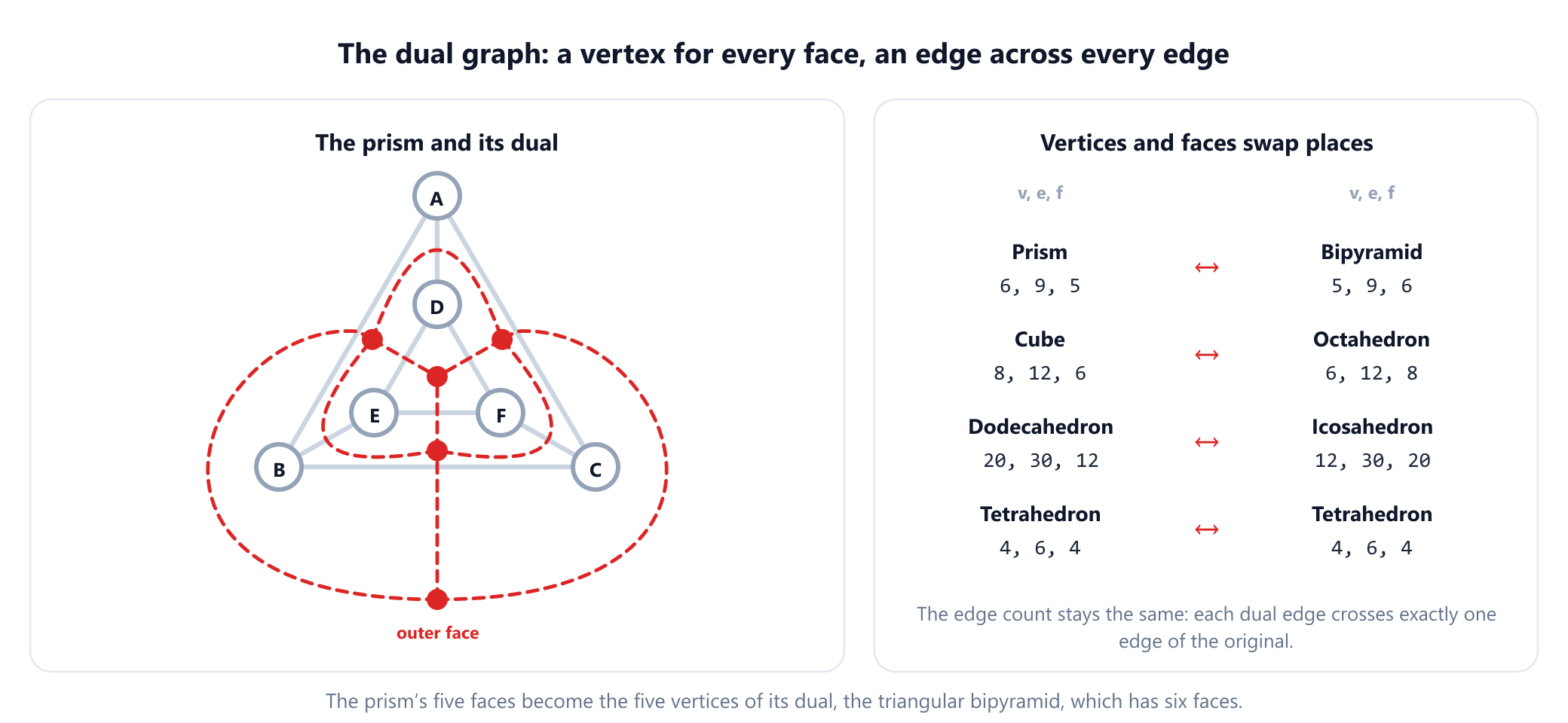
Duality swaps the roles of vertices and faces and keeps the edges: G* has f vertices, e edges and v faces, so Euler's formula reads the same for both. For connected plane graphs the dual of the dual is the original graph again. The Platonic solids pair up under duality, the cube with the octahedron and the dodecahedron with the icosahedron, while the tetrahedron is its own dual.
The dual translates one kind of structure into another:
- Face colouring becomes vertex colouring. Colouring the regions of a map so that neighbours differ is the same as colouring the vertices of the dual graph. This is how the four colour theorem for maps becomes a statement about planar graphs.
- Cycles become cuts. The edges of a cycle in
Gcorrespond to a minimal set of dual edges whose removal disconnectsG*, because the cycle separates the faces inside it from the faces outside. In planar networks this turns a minimum cut problem into a shortest cycle problem in the dual, one of the reasons max flow is faster on planar graphs than in general (see max flow and min cut). - Spanning trees pair up. If
Tis a spanning tree ofG, the duals of the edges not inTform a spanning tree ofG*. Counting edges gives(v − 1) + (f − 1) = e, which is Euler's formula again, from a completely different direction.
One warning goes with the definition. The dual is built from a drawing, not from the graph, so a planar graph with several different embeddings can have several non-isomorphic duals. Whitney proved in 1932 and 1933 that this cannot happen for 3-connected planar graphs, those that stay connected after deleting any two vertices: their embedding on the sphere is essentially unique, and so is their dual. The prism is 3-connected, which is why its dual is well defined. By Steinitz's theorem the 3-connected planar graphs are also exactly the graphs of convex polyhedra, which closes the circle back to Euler.
10. Where planar graphs show up
Planarity is a geometric property, so it appears wherever a network has to be laid out on a surface, and wherever a surface is cut into regions.
| Field | What the graph is | Why planarity matters |
|---|---|---|
| Circuit layout | Components and the connections between them | Wires on one layer of a board or chip cannot cross; a non-planar circuit needs extra layers or jumpers |
| Maps and geography | Regions and shared borders, or the dual of the map | Four colours suffice, and adjacency data stays linear in size |
| Road networks | Junctions and road segments | Almost planar apart from bridges and tunnels, which lets route planners use small separators |
| Meshes and graphics | Vertices, edges and triangles of a surface | Euler's formula gives a cheap sanity check on a closed mesh |
| Computational geometry | Delaunay triangulations, Voronoi diagrams | At most 3n − 6 edges, so the structures have linear size |
| Graph drawing | Any network to be visualised | A crossing-free layout is the most readable one, and Fáry's theorem guarantees straight lines |
Circuits are the classical application. On a single-layer printed circuit board, copper tracks cannot cross without short-circuiting, so the connection graph must be planar. When it is not, designers route some tracks on a second layer and connect the layers through drilled holes called vias, or bridge one track over another with a jumper wire. The minimum number of crossings in any drawing of a graph, its crossing number, measures how badly a circuit fails to be planar, and the number of planar layers needed to hold all its edges is its thickness.
Maps give the second. A map of countries is a plane graph whose faces are the countries, and its dual has one vertex per country and an edge per shared border. Colouring the countries is colouring the dual, and the four colour theorem caps the number of colours at four, provided every country is one connected region. Real atlases break that proviso: a country in separate pieces, such as the United States with Alaska or Russia with Kaliningrad, must have the same colour in two places, and maps with such constraints can need more than four colours.
Road networks and separators give the third. Lipton and Tarjan proved in 1979 that every planar graph with n vertices can be split into two parts, neither larger than 2n/3 vertices, by removing only O(√n) vertices. Small separators are the basis of divide-and-conquer algorithms on planar graphs, including faster shortest path computations. Road networks are not exactly planar, because of bridges and tunnels, but they too can usually be cut into large pieces by removing few junctions, which is the property that partition-based route planners rely on.
Meshes give the last. A closed triangle mesh of a surface shaped like a sphere, with no gaps and no handles, satisfies v − e + f = 2, and since every triangle has three edges and every edge borders two triangles, 3f = 2e. Together these force f = 2v − 4 and e = 3v − 6. A mesh of such a surface that fails these counts has a gap, a missing triangle or a duplicated vertex somewhere, which makes the counts a cheap sanity check when a mesh is imported or repaired.
11. Beyond the plane: crossings and surfaces
A non-planar graph is not the end of the story. Two natural questions measure how far it is from planar.
The first is the crossing number cr(G), the fewest crossings in any drawing. Planar graphs have crossing number 0, and K5 and K3,3 have crossing number 1. Computing it is NP-hard in general, and even for complete graphs exact values are known only for small cases.
The second is to draw on a different surface. A torus, the surface of a ring doughnut, has a hole, and the hole gives edges a way around each other. Both K5 and K3,3 can be drawn on a torus without crossings, and so can K7. Euler's formula generalises: a graph embedded on a surface with g holes, so that every face is a disc, satisfies
v − e + f = 2 − 2g

plane or sphere   g = 0:   v − e + f = 2
torus             g = 1:   v − e + f = 0         K7 on a torus:  7 − 21 + 14 = 0
The number 2 − 2g is the Euler characteristic of the surface, one of the first invariants of topology. Heawood used it in his 1890 paper to bound the number of colours needed on a surface with g holes, and the bound was proved to be exact for every g ≥ 1 by Ringel and Youngs in 1968. For the torus the answer is 7, and K7 shows that seven colours can really be needed. The plane, where the same formula would give 4, was the one case their work did not cover; that was the four colour theorem.
12. Common mistakes
| Mistake | Why it is wrong | Fix |
|---|---|---|
| "My drawing has a crossing, so the graph is not planar" | Planarity asks whether some drawing avoids crossings; K4 has drawings of both kinds | Look for a crossing-free drawing, or prove non-planarity with a bound or a Kuratowski subgraph |
"It satisfies e ≤ 3v − 6, so it is planar" | The bound is necessary only; K3,3 has 9 edges against a limit of 12 | Use the bound only to reject, then run a planarity test |
| Forgetting the outer face | Counting only the enclosed regions gives v − e + f = 1 and makes every later bound wrong | Always count the unbounded face; a tree has exactly one face |
Using v − e + f = 2 on a disconnected graph | The components share one outer face | Use v − e + f = 1 + k for k components |
| Applying the edge bounds to a multigraph | Parallel edges can be added without limit and stay planar | Reduce to the underlying simple graph first; the bounds need a simple graph and v ≥ 3 |
Using 2v − 4 for a graph with triangles | The bound assumes every face has at least four sides | Use 2v − 4 only for triangle-free graphs, such as bipartite ones |
Treating "contains a K5 minor" as "contains a subdivision of K5" | The Petersen graph has a K5 minor but no subdivision of K5 | Quote Wagner's theorem for minors and Kuratowski's for subdivisions |
| "By the four colour theorem every graph needs at most four colours" | The theorem is about planar graphs; K5 needs five | Check planarity before invoking it |
13. Glossary
| Term | Meaning |
|---|---|
| Planar graph | A graph that has at least one drawing in the plane without edge crossings |
| Plane graph, embedding | A specific crossing-free drawing of a planar graph |
| Face | A region of the plane left after removing a plane drawing; exactly one is unbounded |
| Face length | The number of edges on a face's boundary walk, counting an edge twice if the face lies on both its sides |
| Euler's formula | v − e + f = 2 for every connected plane graph |
| Triangulation | A plane graph in which every face is a triangle; it has exactly 3v − 6 edges |
| Girth | The length of a shortest cycle |
| Subdivision | A graph obtained by replacing edges with paths through new vertices of degree 2 |
| Minor | A graph obtained by deleting vertices and edges and contracting edges |
| Kuratowski subgraph | A subdivision of K5 or K3,3, the certificate of non-planarity |
| Dual graph | The graph with a vertex for each face and an edge crossing each edge of a plane graph |
| Rotation system | The cyclic order of edges around every vertex, which determines an embedding |
| Crossing number | The fewest edge crossings in any drawing of a graph in the plane |
14. Frequently asked questions
What is a planar graph?
A planar graph is a graph that can be drawn in the plane so that no two edges cross, with edges meeting only at the vertices they share. Planarity is a property of the graph, not of one picture: a graph is planar if at least one crossing-free drawing exists, even if other drawings of it have crossings. The complete graph K₄ is planar; K₅ and K₃,₃ are not.
What is Euler's formula for planar graphs?
For every connected plane graph, v − e + f = 2, where v is the number of vertices, e the number of edges and f the number of faces, counting the unbounded outer face. The triangular prism, for example, has 6 − 9 + 5 = 2. A plane graph with k components satisfies v − e + f = 1 + k instead.
How do you prove a graph is not planar?
There are two standard ways. By counting: a simple planar graph with v ≥ 3 vertices has at most 3v − 6 edges, and at most 2v − 4 if it has no triangles, so a graph that breaks either bound is not planar. By structure: Kuratowski’s theorem says a graph is non-planar exactly when it contains a subdivision of K₅ or K₃,₃, so exhibiting one is a proof. The counting bounds are necessary conditions only, and a graph that satisfies them can still be non-planar.
Why is K3,3 not planar?
K₃,₃ has 6 vertices and 9 edges, and because it is bipartite it has no triangles, so in a plane drawing every face would need at least 4 edges. Combined with Euler’s formula this limits a triangle-free planar graph on 6 vertices to 2 × 6 − 4 = 8 edges, one fewer than K₃,₃ has. That is why the three utilities puzzle has no solution.
What is the difference between a planar graph and a plane graph?
A planar graph is a graph that can be drawn without crossings. A plane graph is one particular crossing-free drawing, with its faces fixed. The same planar graph can have several plane drawings whose faces have different lengths, but by Euler’s formula every plane drawing of a connected planar graph has the same number of faces.
What does the four colour theorem say?
Every planar graph can be properly coloured with at most four colours, so the regions of any map can be coloured with four colours so that neighbouring regions differ, as long as each region is connected. Appel and Haken proved it in 1976 with the help of a computer; Robertson, Sanders, Seymour and Thomas simplified the proof in 1997, and Gonthier verified it formally in 2005. It applies only to planar graphs: K₅ needs five colours.
15. References
The definitions, theorems and attributions above come from these sources, listed in chronological order.
- Euler, L. (1758). "Elementa doctrinae solidorum." Novi Commentarii Academiae Scientiarum Petropolitanae 4 (1752/53), 109 to 140. The polyhedron formula, stated without proof.
- Euler, L. (1758). "Demonstratio nonnullarum insignium proprietatum, quibus solida hedris planis inclusa sunt praedita." Novi Commentarii Academiae Scientiarum Petropolitanae 4 (1752/53), 140 to 160. Euler's proof by cutting off corners.
- Legendre, A.-M. (1794). Éléments de géométrie. Paris. The first complete proof, by spherical polygons.
- Cauchy, A.-L. (1813). "Recherches sur les polyèdres. Premier mémoire." Journal de l'École Polytechnique 9 (16e cahier), 68 to 86.
- Kempe, A. B. (1879). "On the Geographical Problem of the Four Colours." American Journal of Mathematics 2(3), 193 to 200.
- Heawood, P. J. (1890). "Map-Colour Theorem." Quarterly Journal of Pure and Applied Mathematics 24, 332 to 338. The flaw in Kempe's proof, the five colour theorem, and the bound for other surfaces.
- Dudeney, H. E. (1917). Amusements in Mathematics. London: Thomas Nelson. Problem 251, "Water, Gas, and Electricity."
- Steinitz, E. (1922). "Polyeder und Raumeinteilungen." In Encyklopädie der mathematischen Wissenschaften, Band 3 (Geometrie), Teil 3AB12, 1 to 139. Leipzig: Teubner.
- Kuratowski, K. (1930). "Sur le problème des courbes gauches en topologie." Fundamenta Mathematicae 15, 271 to 283.
- Whitney, H. (1932). "Non-separable and Planar Graphs." Transactions of the American Mathematical Society 34(2), 339 to 362. Combinatorial duals.
- Whitney, H. (1933). "2-Isomorphic Graphs." American Journal of Mathematics 55, 245 to 254. Uniqueness of the embedding of 3-connected planar graphs.
- Wagner, K. (1936). "Bemerkungen zum Vierfarbenproblem." Jahresbericht der Deutschen Mathematiker-Vereinigung 46, 26 to 32. Straight-line drawings.
- Wagner, K. (1937). "Über eine Eigenschaft der ebenen Komplexe." Mathematische Annalen 114, 570 to 590. Planarity by forbidden minors.
- Fáry, I. (1948). "On Straight Line Representation of Planar Graphs." Acta Scientiarum Mathematicarum (Szeged) 11, 229 to 233.
- Grötzsch, H. (1959). "Zur Theorie der diskreten Gebilde, VII: Ein Dreifarbensatz für dreikreisfreie Netze auf der Kugel." Wissenschaftliche Zeitschrift der Martin-Luther-Universität Halle-Wittenberg, Mathematisch-Naturwissenschaftliche Reihe 8, 109 to 120.
- Ringel, G. and Youngs, J. W. T. (1968). "Solution of the Heawood Map-Coloring Problem." Proceedings of the National Academy of Sciences 60(2), 438 to 445.
- Hopcroft, J. and Tarjan, R. (1974). "Efficient Planarity Testing." Journal of the ACM 21(4), 549 to 568.
- Garey, M. R., Johnson, D. S. and Stockmeyer, L. (1976). "Some Simplified NP-Complete Graph Problems." Theoretical Computer Science 1(3), 237 to 267. Planar 3-colourability is NP-complete.
- Lakatos, I. (1976). Proofs and Refutations: The Logic of Mathematical Discovery. Edited by J. Worrall and E. Zahar. Cambridge: Cambridge University Press.
- Appel, K. and Haken, W. (1977). "Every Planar Map is Four Colorable. Part I: Discharging." Illinois Journal of Mathematics 21(3), 429 to 490.
- Appel, K., Haken, W. and Koch, J. (1977). "Every Planar Map is Four Colorable. Part II: Reducibility." Illinois Journal of Mathematics 21(3), 491 to 567.
- Lipton, R. J. and Tarjan, R. E. (1979). "A Separator Theorem for Planar Graphs." SIAM Journal on Applied Mathematics 36(2), 177 to 189.
- Federico, P. J. (1982). Descartes on Polyhedra: A Study of the De Solidorum Elementis. New York: Springer. Descartes's manuscript and Leibniz's copy.
- de Fraysseix, H. and Rosenstiehl, P. (1985). "A Characterization of Planar Graphs by Trémaux Orders." Combinatorica 5(2), 127 to 135. The left-right criterion.
- Robertson, N., Sanders, D. P., Seymour, P. and Thomas, R. (1997). "The Four-Colour Theorem." Journal of Combinatorial Theory, Series B 70(1), 2 to 44.
- Boyer, J. M. and Myrvold, W. J. (2004). "On the Cutting Edge: Simplified O(n) Planarity by Edge Addition." Journal of Graph Algorithms and Applications 8(3), 241 to 273.
- Robertson, N. and Seymour, P. D. (2004). "Graph Minors. XX. Wagner's Conjecture." Journal of Combinatorial Theory, Series B 92(2), 325 to 357.
- Gonthier, G. (2008). "Formal Proof: The Four-Color Theorem." Notices of the American Mathematical Society 55(11), 1382 to 1393.
- Bondy, J. A. and Murty, U. S. R. (2008). Graph Theory. Graduate Texts in Mathematics 244. Springer. Chapters 10 and 11 on planar graphs and the four colour problem.
- Diestel, R. (2017). Graph Theory, 5th edition. Graduate Texts in Mathematics 173. Berlin: Springer. Chapter 4 on planar graphs.
From faces to colours
Build a planar graph, colour it, and check the count against the four colour theorem. Then add the edges of K₅ and watch a fifth colour become unavoidable.
Open the visualizer