
Table of Contents
- 1. What graph theory actually studies
- 2. The definition, and what it leaves out on purpose
- 3. Where it started: seven bridges and one impossible walk
- 4. The vocabulary, and the first theorem
- 5. The families of graphs
- 6. Walks, trails, paths and cycles
- 7. Connectivity, components and the edges you cannot lose
- 8. Trees: the most useful special case
- 9. How a graph is stored in a computer
- 10. Traversal: breadth first and depth first
- 11. The classic problems and their algorithms
- 12. Five results worth knowing by name
- 13. What is easy, what is hard, and why it matters
- 14. Where graphs actually show up
- 15. Mistakes beginners reliably make
- 16. Where to go next
- 17. Glossary
- 18. Frequently asked questions
- 19. References
1. What graph theory actually studies
Graph theory is the study of one very small idea: a collection of objects, and a record of which pairs of them are connected. That is the whole subject. What makes it worth a century and a half of mathematics is that an enormous number of practical questions turn out to be questions about exactly that, and nothing else.
Consider four problems that look unrelated. A delivery company wants the shortest route between two depots. A compiler needs the order in which to build a project's modules. A biologist wants to know which proteins interact, directly or through intermediaries. A network operator wants to know which cable, if cut, would isolate a region. These have nothing in common as stories. Structurally they are the same handful of problems asked about the same kind of object, and the algorithms that answer them are interchangeable. That transferability is why the subject is taught early and used everywhere: once a situation is written as a graph, a large catalogue of results becomes available at once, and none of them care what the vertices originally represented.
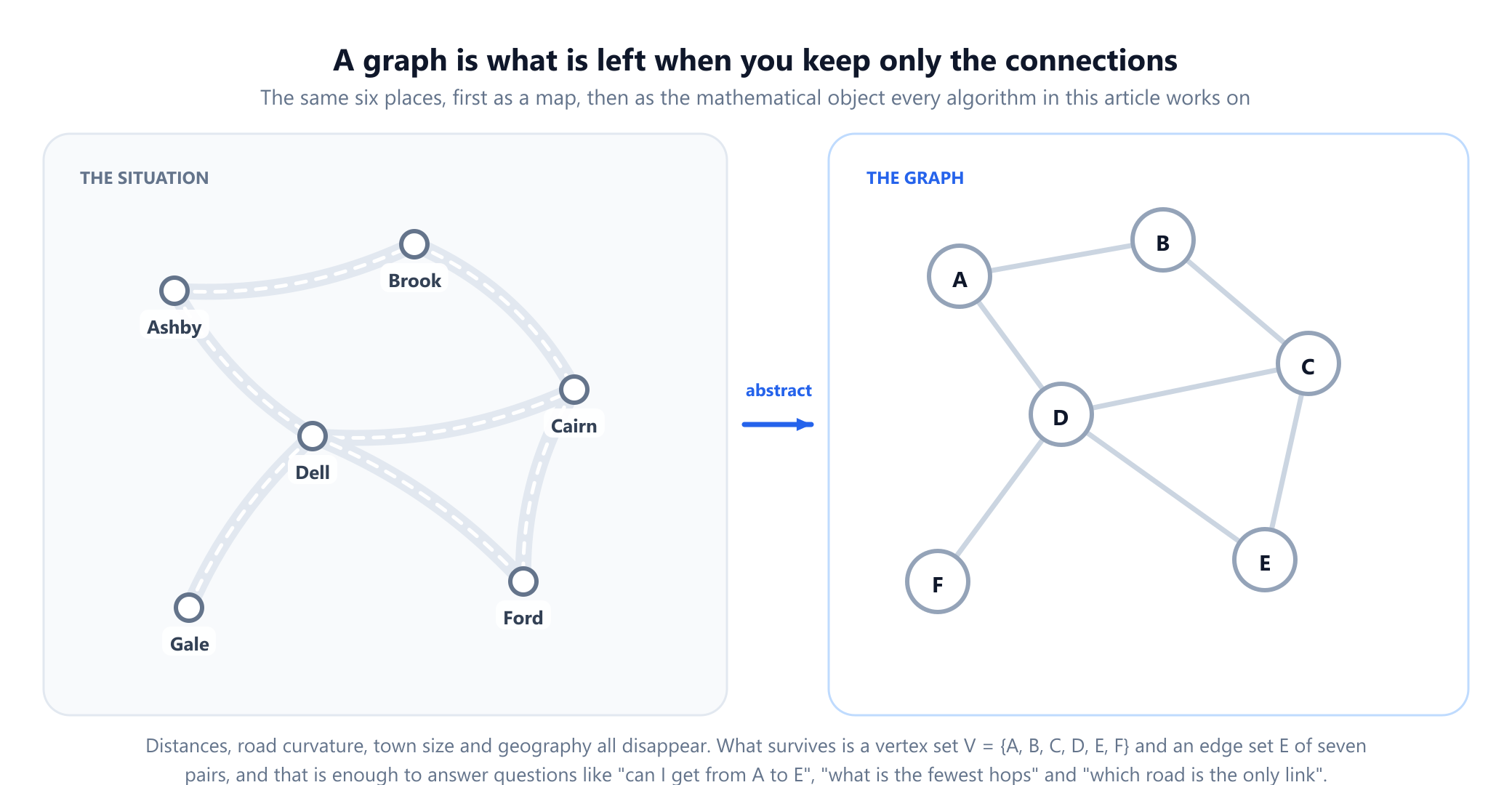
Notice what the picture on the right does not contain. The towns have moved, the roads are straight, and nothing records that one is twice as long as another. If those facts matter for your question you must add them back explicitly, as numbers on the edges. If they do not, throwing them away is exactly what makes the problem tractable.
This article is a first course in one page: the definitions in order, the small results everything else rests on, how graphs are stored and searched in real code, the classic problems, and an honest map of which questions a computer can answer in seconds and which it cannot answer at all. Each section links to a deeper article if you want more on that one topic.
2. The definition, and what it leaves out on purpose
Almost every popular account says a graph is "dots joined by lines". That picture is useful, and it is also why many people get stuck a few weeks later: the dots and the lines are a drawing of the object, not the object. The object is a pair of sets. Diestel's Graph Theory, the standard graduate reference, states it in its cleanest form:
A graph is a pair G = (V, E) of sets such that E ⊆ [V]2, where [V]2 is the set of all 2-element subsets of V.
Unpacked, that says four things:
- V is a set of objects, called vertices (or nodes). Nothing at all is assumed about them. They may be cities, people, atoms, web pages or integers. The theory never looks inside a vertex; it only needs to be able to tell two of them apart.
- E is a set of 2-element subsets of V. An edge is literally the set
{u, v}. It is not an arrow, not a curve, and it carries no information beyond which pair it joins. - Because E is a set, an edge is either present or absent. It cannot appear twice.
- Because each edge has two distinct members, no edge joins a vertex to itself.
Those last two consequences are not extra rules somebody added; they fall straight out of the set theory, and a graph obeying them is called simple. Allowing repeated edges or self-loops means changing the definition itself, which is what multigraphs do in section 5.
Two more pieces of notation appear everywhere. Write V(G) and E(G) when several graphs are in play. And the two size measures have names: the number of vertices is the order of the graph, the number of edges is its size, abbreviated in nearly all algorithm texts to n = |V| and m = |E|.
What the definition leaves out is as informative as what it includes. There is no geometry, so two drawings of the same graph are the same graph even if one looks like a spiral and the other like a grid. There is no order on the vertices. There are no distances, capacities or costs; those come from an extra function, usually written w: E → ℝ, bolted on when a problem needs it. The bare object is deliberately impoverished, and that poverty is what makes theorems about it apply so widely. The companion guide on vertices and edges works the same definition through in more detail.
3. Where it started: seven bridges and one impossible walk
The subject has a birthday. In 1736 Leonhard Euler, then at the St Petersburg Academy, sent in a paper titled Solutio problematis ad geometriam situs pertinentis, "the solution of a problem relating to the geometry of position". The problem came from the Prussian city of Königsberg, now Kaliningrad. The river Pregel divided the city into four land masses, joined by seven bridges, and the citizens amused themselves with a question: can you walk through the city crossing every bridge exactly once?
Euler's first move is the move this whole article is about. The size and shape of the land masses are irrelevant, the length of the bridges is irrelevant, and the only thing that matters is which land mass connects to which, and how many times. Strip the rest and you have four objects and seven connections, which modern textbooks draw as a multigraph with four vertices and seven edges.
His argument is short enough to give in full. Suppose the walk exists, and take any land mass that is not its start or end. Every time the walk arrives there it must also leave, so the bridges at that land mass are used in pairs and their number must be even. In Königsberg the four land masses had 5, 3, 3 and 3 bridges, all odd. A walk has only two ends, so at most two land masses may have an odd count. Four is too many, and no such walk exists.
Why this argument matters more than the answer. Euler did not search for a route and fail. He proved that no route can exist, by counting a quantity that any successful route would have to respect. That style of reasoning, find an invariant, show the goal violates it, is what separates graph theory from puzzle solving, and it is why 1736 counts as the start of a field rather than the solution of a riddle.
Euler stated the converse too, but did not prove it; that gap stayed open until Carl Hierholzer gave a constructive proof, published posthumously in 1873. The modern statement is clean: a connected graph has a closed walk using every edge exactly once, an Eulerian circuit, if and only if every vertex has even degree, and an open one, an Eulerian trail, if and only if exactly two vertices have odd degree. The full story is in the guide to the Eulerian path and circuit.
The century that followed filled in the foundations, from Kirchhoff's spanning trees in 1847 to Sylvester borrowing the word "graph" from chemistry in 1878 and König's first textbook in 1936. That story is told in the history of graph theory.
4. The vocabulary, and the first theorem
The rest of this article uses one running example, a graph with seven vertices and eight edges. It is small enough to check every claim by hand and large enough to be interesting.
V = {A, B, C, D, E, F, G}                          n = 7
E = { {A,B}, {A,C}, {B,C}, {B,D}, {C,E},
      {D,E}, {D,F}, {F,G} }                        m = 8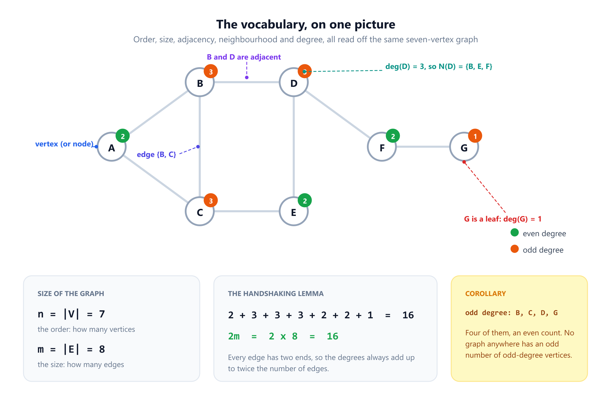
Here are the terms, each one defined only from the two sets:
- Adjacent. Two vertices joined by an edge. B and D are adjacent, A and D are not.
- Incident. An edge is incident to each of its two endpoints. Adjacency relates a vertex to a vertex, incidence relates a vertex to an edge, and beginners routinely swap the two.
- Neighbourhood.
N(v), the set of vertices adjacent to v. HereN(D) = {B, E, F}. - Degree.
deg(v), the number of edge ends meeting v, which in a simple graph is just|N(v)|. Heredeg(B) = 3anddeg(G) = 1. - Leaf and isolated vertex. Degree 1, such as G, and degree 0. Isolated vertices are legal, and they are the most commonly lost piece of data when a graph is built from an edge list, because an edge list has no way to mention them.
- Minimum and maximum degree.
δ(G)andΔ(G), here 1 at G and 3 at B, C and D.
With degree defined, the first theorem is one line away. The seven degrees sum to 2 + 3 + 3 + 3 + 2 + 2 + 1 = 16, exactly twice the eight edges, and that is not a coincidence about this graph.
The handshaking lemma. In any graph, the sum of all vertex degrees equals twice the number of edges.
Proof: count the pairs (v, e) where the vertex v is an endpoint of the edge e. Counting by vertices gives the sum of the degrees. Counting by edges gives 2m, because every edge has exactly two ends. Two counts of the same set must agree.
That technique, counting one collection in two ways, is called double counting, and it is the workhorse of elementary combinatorics. The lemma has a corollary that surprises people the first time: the number of vertices of odd degree is always even. Here they are B, C, D and G, which is four. The reason is arithmetic: the total is even and the even-degree vertices contribute an even amount, so the odd-degree vertices must contribute an even amount between them, which takes an even number of them. In everyday terms, the number of people in a room who have shaken hands an odd number of times is even. Euler's Königsberg argument is this corollary applied to a walk.
5. The families of graphs
The bare definition in section 2 is the most restrictive one. Every real modelling problem eventually needs a variation, and each variation is a specific, named change to what an edge is allowed to be. Knowing which family you are in decides which algorithms are even applicable, so this is not vocabulary for its own sake.
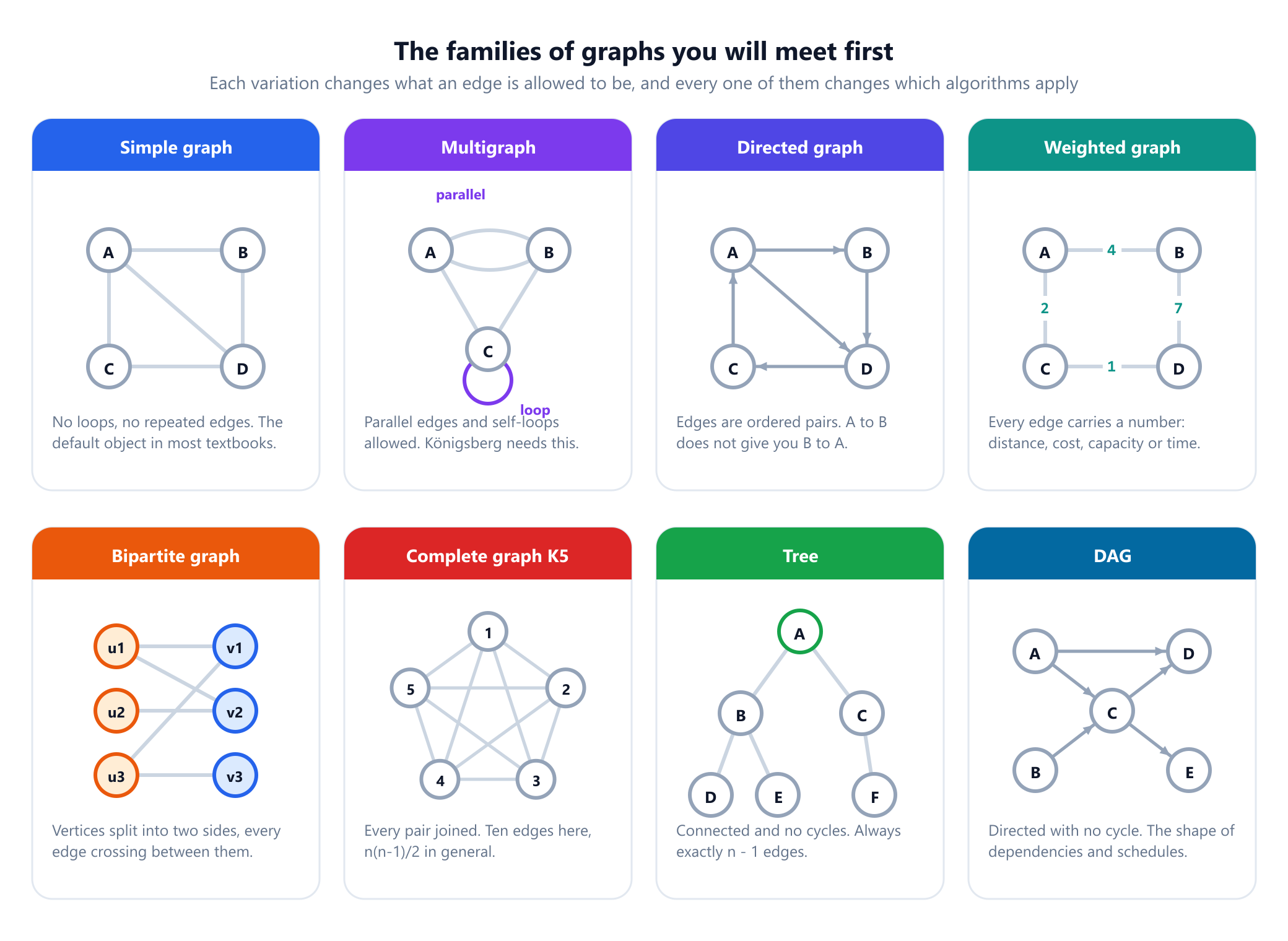
Simple graphs are the default: no loops, no repeated edges, and every unqualified result in a textbook is about these. Multigraphs allow parallel edges and pseudographs allow self-loops too. Königsberg genuinely needs a multigraph, since two of its land masses were joined by two bridges, and a loop adds 2 to the degree of its vertex because both ends attach there. See simple graphs versus multigraphs.
Directed graphs, or digraphs, replace the unordered pair {u, v} with the ordered pair (u, v), called an arc, so a digraph may contain either direction, both or neither, and degree splits into in-degree and out-degree. This is the right model whenever the relation is not symmetric: one way streets, "A follows B", "module A imports module B", "task A must finish before task B". See directed versus undirected graphs.
Weighted graphs add a function w assigning a number to each edge: kilometres, minutes, price, capacity, similarity. Algorithms have strong opinions about those numbers. Dijkstra's algorithm requires them to be non-negative, Bellman-Ford tolerates negatives but not negative cycles, and breadth first search ignores them entirely, which is why running BFS on a weighted graph and calling the result a shortest path is one of the most common bugs in beginner code. See weighted versus unweighted graphs.
Bipartite graphs split the vertex set into two parts with every edge running between them. Students and courses, applicants and jobs, buyers and products: any two sided matching situation is bipartite. A graph is bipartite exactly when it contains no odd cycle, and a single breadth first search that two-colours the vertices decides it in linear time.
Complete graphs, written Kn, have every possible edge. Since an edge is a choice of 2 vertices from n, the count is n(n-1)/2, so K5 has 10 edges and K100 has 4,950. That is also the ceiling for any simple graph on n vertices, and it is what the density of a graph is measured against.
Trees are connected graphs with no cycles, the subject of section 8. DAGs, directed acyclic graphs, are digraphs with no directed cycle, and they are the shape of every dependency and every schedule: spreadsheet formulas, build targets, Git commits and the operations of a neural network are all DAGs, and the algorithm that puts them in a valid order is topological sorting.
One more is worth knowing by name: planar graphs can be drawn with no edges crossing, which matters for circuit layout and map colouring, and which section 12 returns to.
6. Walks, trails, paths and cycles
Four words describe movement through a graph, they are used interchangeably in casual speech, and they mean four different things. Getting them straight prevents a surprising amount of confusion later, because theorems are stated with the precise word and the difference between them is often the entire content of the result.
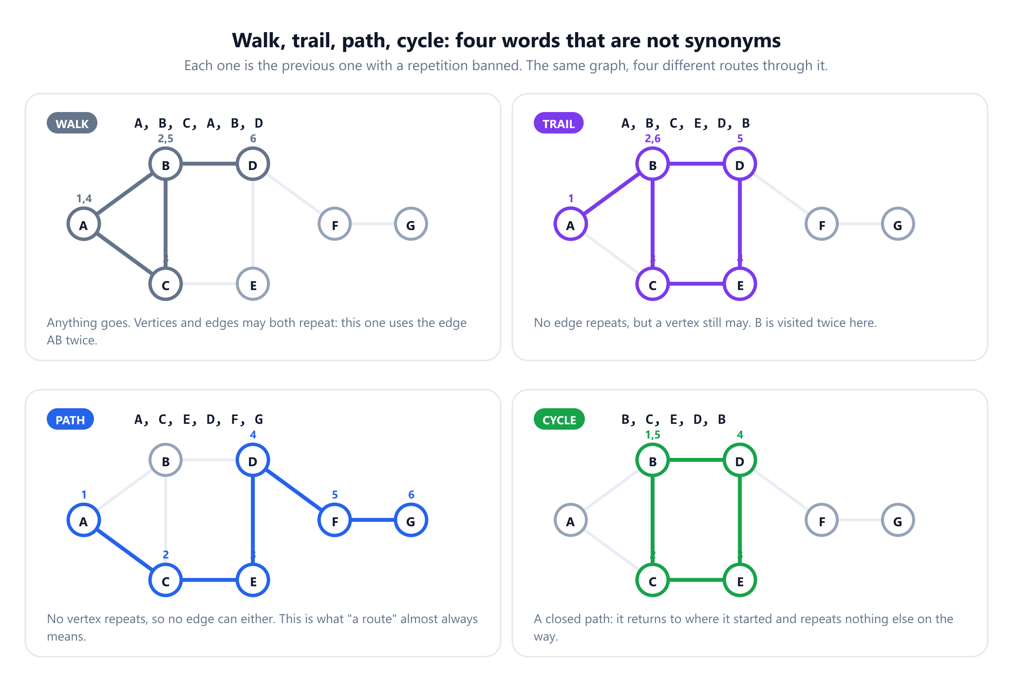
- A walk is any sequence of vertices where consecutive ones are adjacent. Nothing is forbidden. A walk may cross the same edge and revisit the same vertex as often as it likes.
- A trail is a walk with no repeated edge. Vertices may still repeat. Euler's bridge problem asks for a trail that uses every edge, which is why it is an Eulerian trail and not an Eulerian path.
- A path is a walk with no repeated vertex, which automatically forbids repeated edges too. When somebody says "the route from A to G", this is what they mean.
- A cycle is a closed path: it starts and ends at the same vertex and repeats nothing else. In the example, B, C, E, D, B is a cycle of length 4, and A, B, C, A is a triangle, a cycle of length 3.
The length of any of these is its number of edges, not its number of vertices, which is an off-by-one waiting to happen. The distance d(u, v) is the length of a shortest path. Here d(A, G) = 4, along A, B, D, F, G; the route A, C, E, D, F, G also arrives but uses five edges, so it is a path and not a shortest one. The diameter is the largest distance between any pair of vertices, a compact way of saying how spread out a network is.
One fact follows immediately and gets used constantly: if there is a walk from u to v, there is a path from u to v. Cut out the loop between any two visits to the same vertex and the result is a shorter walk, so the surgery ends at one with no repeated vertex. This is why reachability algorithms never consider walks at all.
7. Connectivity, components and the edges you cannot lose
A graph is connected when every vertex can be reached from every other. When it is not, it falls apart into connected components, which are the maximal pieces that are internally connected. Connectivity is the first thing worth checking about any graph you did not construct yourself, because a surprising number of real datasets arrive in several pieces and most reported bugs of the form "the algorithm returned infinity" are that fact discovered the hard way.
Within a connected graph, some parts of the structure are more critical than others. A bridge is an edge whose removal increases the number of components, and a cut vertex, or articulation point, is a vertex whose removal does the same. These are the single points of failure, and finding them is the standard first analysis of any network whose reliability matters.
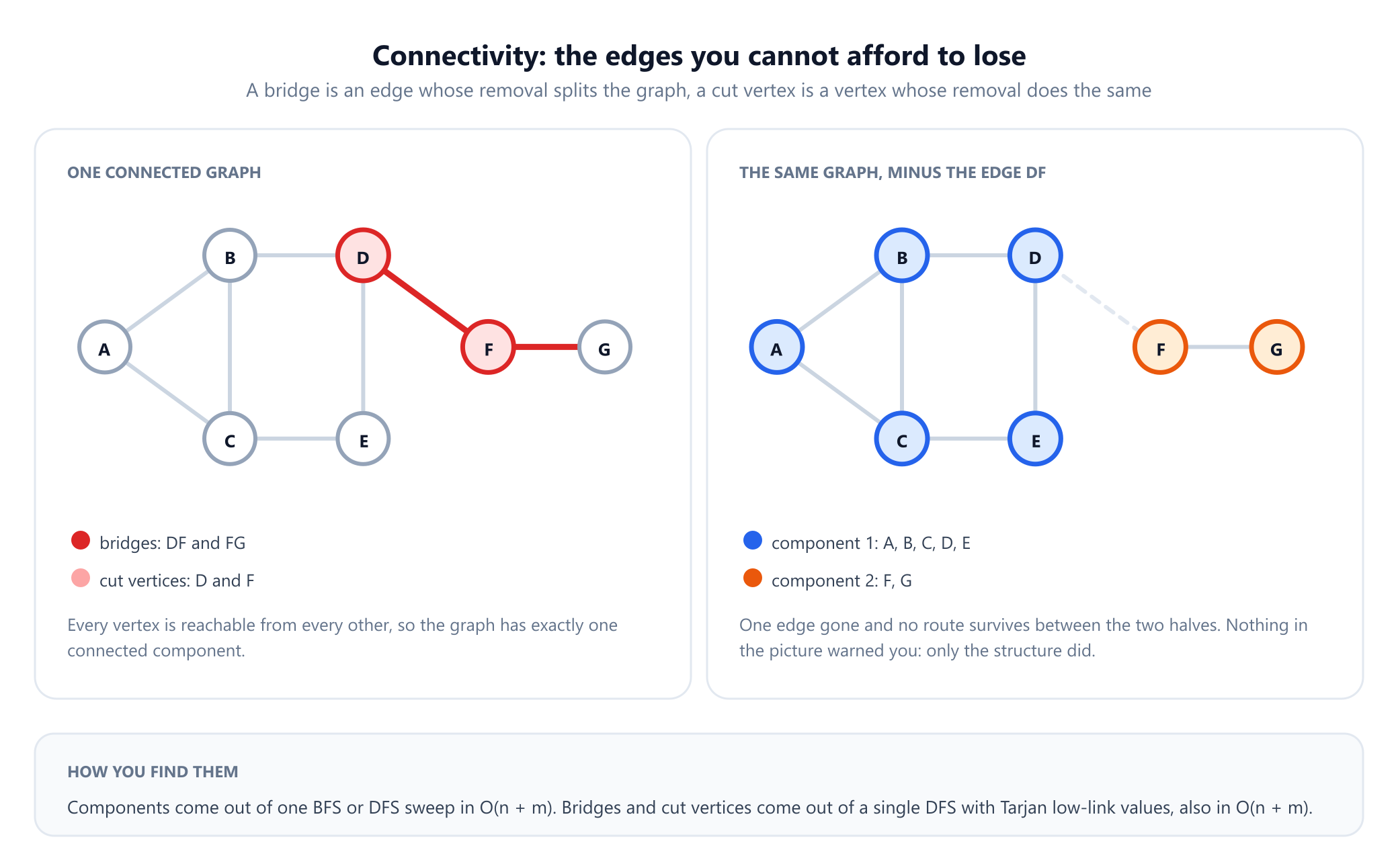
In the running example the edges DF and FG are bridges, and D and F are cut vertices. Note what is not a bridge: none of the five edges that lie on a cycle, because a cycle always offers a detour. That is the general rule, and it is worth stating as a fact rather than an observation. An edge is a bridge exactly when it lies on no cycle. The same intuition explains why redundancy in real networks is measured in cycles: a second route is a cycle through the first.
For directed graphs the notion splits in two: a digraph is weakly connected if ignoring arc directions leaves a connected graph, and strongly connected if every vertex reaches every other by following arcs the right way round. Tarjan's 1972 algorithm finds the strongly connected components in linear time, and in a dependency graph one with more than a single vertex is precisely a circular dependency.
Computationally all of this is cheap. One breadth first or depth first sweep labels every component in O(n + m), and bridges and cut vertices come out of a single depth first search augmented with Tarjan's low-link values, also in O(n + m). There is rarely a reason not to check connectivity before doing anything else.
8. Trees: the most useful special case
A tree is a connected graph with no cycles. It is the single most important special case in the subject, partly because trees show up everywhere in computing and partly because a great many hard problems become easy when the input happens to be one.
What makes trees remarkable is how many different-sounding descriptions pick out the same objects. For a graph G on n vertices, all of the following are equivalent, and any one can serve as the definition:
- G is connected and has no cycles.
- G is connected and has exactly
n - 1edges. - G has no cycles and has exactly
n - 1edges. - Between every pair of vertices there is exactly one path.
- G is connected, and removing any edge disconnects it, so every edge is a bridge.
- G has no cycles, and adding any new edge creates exactly one cycle.
The equivalence is proved as a cycle of implications, laid out in the guide to trees in graph theory. Two consequences are worth carrying around. The edge count is forced, so a "tree" with 100 vertices and 120 edges is not a tree and something upstream is wrong. And uniqueness of paths is why tree problems are easy: there is nothing to search for, because there is only ever one route.
A forest is an acyclic graph that need not be connected, so it is a disjoint union of trees, and one with n vertices and c components has exactly n - c edges. A spanning tree of a connected graph is a tree subgraph containing every vertex, the cheapest skeleton that keeps the graph in one piece. Both traversals produce one for free as a side effect, and when edges carry weights, finding the lightest is the minimum spanning tree problem.
Trees also come in a rooted flavour, where one vertex is singled out and the words parent, child, ancestor, subtree and depth become available, as in file systems, parse trees and heaps. Rooting is a choice laid on top of the graph rather than a property of it, which is the point of the article on rooted trees.
9. How a graph is stored in a computer
Everything so far has been mathematics. The moment a machine has to answer a question about a graph, you must choose how it is laid out in memory, and that choice is not an implementation detail: it changes which operations are cheap by factors of thousands, and a badly matched representation is the most common reason a correct algorithm runs too slowly. There are three standard layouts, and they store exactly the same information.
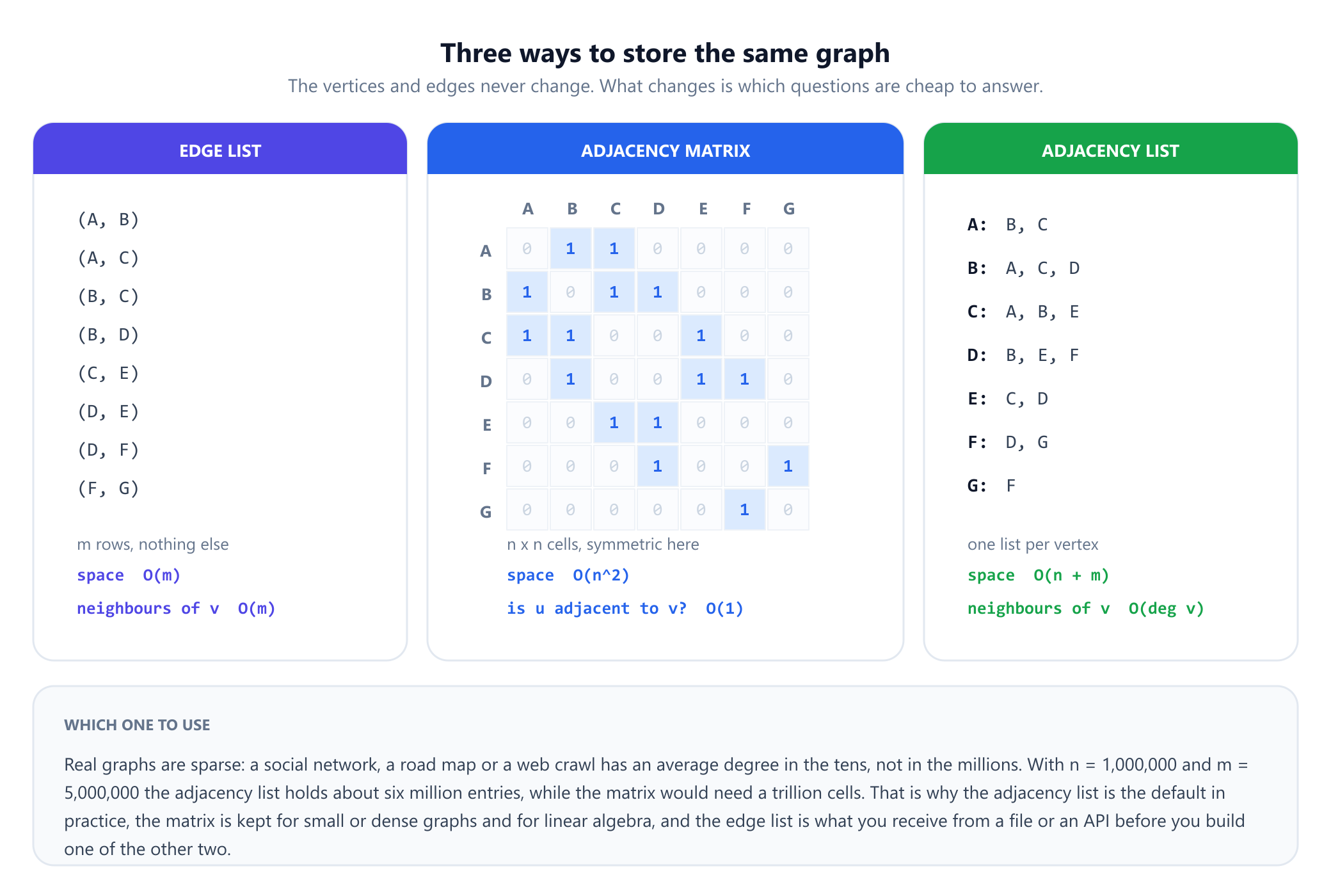
The edge list is the set E written out. It is compact, it is what a CSV file or an API hands you, and it is what Kruskal's algorithm wants, since that algorithm sorts edges by weight and never asks about a particular vertex. Its weakness is that "who are the neighbours of D" means scanning all m rows.
The adjacency matrix is an n by n grid where cell (u, v) is 1 when the edge is present. Checking whether two given vertices are adjacent is a single lookup, and for undirected graphs the matrix is symmetric, so it stores every fact twice. The cost is space: n squared cells whether or not there are any edges. It is also the gateway to spectral methods, where the eigenvalues of the matrix, or of the closely related Laplacian, expose clustering and connectivity, the subject of spectral graph theory in machine learning.
The adjacency list keeps, for each vertex, the list of its neighbours. Iterating over the neighbours of v costs O(deg v), which is optimal, and the total space is O(n + m). This is the default in practice, and the layout every traversal below assumes.
| Operation | Edge list | Adjacency matrix | Adjacency list |
|---|---|---|---|
| Space | O(m) | O(n2) | O(n + m) |
| Is u adjacent to v? | O(m) | O(1) | O(deg u) |
| Visit all neighbours of u | O(m) | O(n) | O(deg u) |
| Add an edge | O(1) | O(1) | O(1) |
| Delete an edge | O(m) | O(1) | O(deg u) |
| Iterate over all edges | O(m) | O(n2) | O(n + m) |
What decides the argument in practice is that real networks are sparse: the average number of neighbours stays in the tens no matter how large the network grows, since junctions have three or four roads and people have a bounded number of friends. For a graph with a million vertices and five million edges the adjacency list holds about ten million entries, while the matrix would need a trillion cells, several terabytes for a graph that otherwise fits comfortably in memory. Use the matrix when the graph is small, genuinely dense, or destined for linear algebra; use the adjacency list otherwise. The deeper treatment, including compressed sparse row layouts, is in graph representation.
Building an adjacency list from an edge list takes four lines, and the comment in the middle is the part beginners get wrong:
edges = [('A','B'), ('A','C'), ('B','C'), ('B','D'),
         ('C','E'), ('D','E'), ('D','F'), ('F','G')]

graph = {v: [] for v in 'ABCDEFG'}   # start from V, so isolated vertices survive
for u, v in edges:
    graph[u].append(v)
    graph[v].append(u)               # omit this line for a directed graph
Starting from the vertex set rather than the edges is what keeps isolated vertices in the graph. Build the dictionary lazily from the edge list and any vertex with no edges silently disappears, changing n and breaking every calculation that divides by it.
10. Traversal: breadth first and depth first
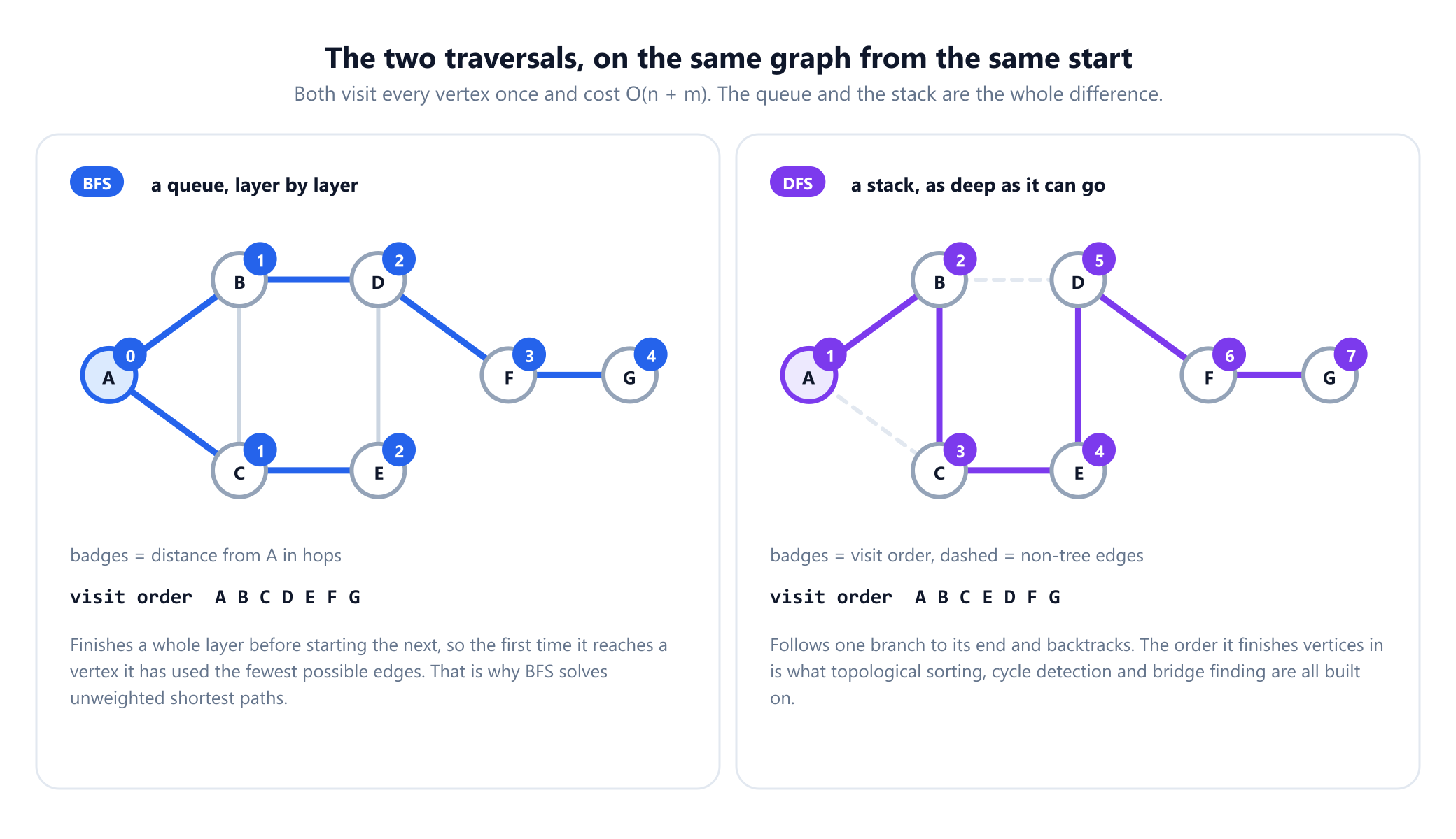
Almost every graph algorithm is a traversal with bookkeeping attached. There are two, they differ by one data structure, and understanding that difference is the highest-value hour a beginner can spend on the subject. Both start at a vertex, keep a collection of vertices discovered but not yet processed, and repeat: take one out, look at its neighbours, add the new ones. Breadth first search takes them out in the order they went in, using a queue. Depth first search takes out the most recently added, using a stack or the call stack of a recursive function. That single choice produces two completely different shapes of exploration.
Here is breadth first search in full, returning the visit order, the distance from the start and the tree of parents that lets you reconstruct the actual routes:
from collections import deque

def bfs(graph, start):
    dist = {start: 0}
    parent = {start: None}
    queue = deque([start])
    order = []
    while queue:
        u = queue.popleft()          # a queue: first in, first out
        order.append(u)
        for v in graph[u]:
            if v not in dist:        # not yet discovered
                dist[v] = dist[u] + 1
                parent[v] = u
                queue.append(v)
    return order, dist, parent

order, dist, parent = bfs(graph, 'A')
# order  ['A', 'B', 'C', 'D', 'E', 'F', 'G']
# dist   {'A': 0, 'B': 1, 'C': 1, 'D': 2, 'E': 2, 'F': 3, 'G': 4}
The important property is in the dist dictionary. Because BFS finishes an entire layer before starting the next, the first time it reaches a vertex it has used the fewest possible edges, so BFS solves the shortest path problem on unweighted graphs in O(n + m). Reaching for Dijkstra when every edge costs the same is wasted work.
Depth first search is the same skeleton with a stack instead of a queue:
def dfs(graph, start):
    seen = set()
    order = []
    stack = [start]
    while stack:
        u = stack.pop()              # a stack: last in, first out
        if u in seen:
            continue
        seen.add(u)
        order.append(u)
        for v in reversed(graph[u]): # reversed, so the first neighbour is taken first
            if v not in seen:
                stack.append(v)
    return order

dfs(graph, 'A')   # ['A', 'B', 'C', 'E', 'D', 'F', 'G']
DFS does not give you distances, and the order in which it finishes vertices is the useful output rather than the order in which it starts them. That finishing order is what topological sorting, cycle detection, strongly connected components and bridge finding are all built from, following Tarjan's 1972 paper that turned depth first search from a technique into a toolkit.
The one thing to remember. Use BFS when the question is about distance or the fewest steps, and DFS when the question is about structure: does a cycle exist, what depends on what, which pieces hang together. Both cost O(n + m) and both visit every vertex exactly once, so the choice is never about speed.
A fuller comparison of the two, including the bugs each one invites, is in BFS versus DFS.
11. The classic problems and their algorithms
With traversal in place, the standard catalogue is within reach. Each of these is a question people genuinely ask about real networks, and each has a named algorithm.
Shortest paths. Unweighted, BFS answers it. With non-negative weights, Dijkstra's algorithm, published in a three page note in 1959, settles vertices in increasing order of distance and runs in O(m + n log n) with a good priority queue. With negative weights, Dijkstra's central assumption fails and you need Bellman-Ford, which relaxes every edge n-1 times in O(nm) and detects negative cycles as a bonus. For every pair at once, Floyd-Warshall does it in O(n3) with three nested loops, and when you have a goal and a sensible estimate of the distance remaining, A* search uses it to examine a fraction of the graph. The full decision tree is in shortest path algorithms.
Minimum spanning trees. Find the cheapest set of edges that keeps a weighted graph connected. Kruskal's algorithm sorts the edges and adds any that does not close a cycle, using a union-find structure to test that in near constant time; Prim's grows one tree outward, always taking the cheapest edge leaving it. Both are greedy, both are provably optimal, and both run in O(m log n). This is the algorithm behind laying cable and fibre at minimum cost, and it appears inside clustering methods too.
Ordering and flow. Given a DAG of dependencies, topological sorting produces an order in which every task follows what it depends on, in O(n + m), failing exactly when a cycle exists. Given pipes with capacities, maximum flow asks how much can move from a source to a sink; formalised by Ford and Fulkerson in 1956, it models traffic, bandwidth, supply chains and, through a standard reduction, bipartite matching. See network flow, max-flow and min-cut.
Colouring. Label the vertices so that no two adjacent ones share a label, using as few labels as possible. That count is the chromatic number, and it models exam timetabling, frequency assignment and register allocation. Unlike everything above, this one is NP-hard and practice relies on heuristics. See the graph colouring problem.
Tours. A Hamiltonian cycle visits every vertex exactly once, and the travelling salesperson problem asks for the cheapest one. It looks like a small variation on Euler's question from 1736, which is linear time, and it is among the hardest problems in the catalogue. Its practical cousin, routing a fleet from a depot under capacity limits, is the vehicle routing problem.
| Problem | Algorithm | Complexity | Requires |
|---|---|---|---|
| Reachability, components | BFS or DFS | O(n + m) | Nothing |
| Shortest path, unweighted | BFS | O(n + m) | Nothing |
| Shortest path, weighted | Dijkstra | O(m + n log n) | No negative weights |
| Shortest path, negative weights | Bellman-Ford | O(nm) | No negative cycles |
| All pairs shortest paths | Floyd-Warshall | O(n3) | No negative cycles |
| Minimum spanning tree | Kruskal or Prim | O(m log n) | Undirected, connected |
| Task ordering | Topological sort | O(n + m) | Directed and acyclic |
| Maximum flow | Dinic, Orlin | O(nm) and better | Capacities |
| Bipartite matching | Hopcroft-Karp | O(m√n) | Bipartite |
| Minimum colouring | None known | Exponential | NP-hard |
| Cheapest tour (TSP) | Held-Karp, heuristics | O(n22n) exact | NP-hard |
12. Five results worth knowing by name
A first course is partly a set of algorithms and partly a set of results that shape how you think about the objects. The handshaking lemma from section 4 is the first of them. These five come up just as constantly, in interviews, in papers and in conversation, and each can be stated in a sentence.
Euler's criterion for traversing every edge (1736, completed by Hierholzer in 1873)
A connected graph has a closed trail using every edge exactly once if and only if every vertex has even degree, and an open one if and only if exactly two vertices have odd degree. This is the valuable kind of theorem: it turns a search over an enormous space of routes into a check you can do by counting, in linear time.
Euler's formula for planar graphs (1758)
Draw a connected planar graph with no crossings and let f be the number of faces, counting the unbounded outer region. Then
n - m + f = 2The running example, drawn as in the figures, has n = 7, m = 8 and three faces: the triangle ABC, the quadrilateral BCED and the outer region, and indeed 7 - 8 + 3 = 2. The corollary has real teeth: any simple planar graph with at least three vertices satisfies m ≤ 3n - 6, so planar graphs are always sparse, and K5 with its 5 vertices and 10 edges cannot be planar since 3n - 6 is 9. Kuratowski's theorem of 1930 completes the picture: a graph is planar exactly when it contains no subdivision of K5 or K3,3. Hopcroft and Tarjan showed in 1974 that planarity can be tested in linear time.
The four colour theorem (Appel and Haken, 1976)
Every planar graph can be properly coloured with at most four colours, so no map needs more than four colours for countries sharing a border to differ. Francis Guthrie asked the question in 1852 and it resisted proof for 124 years. The eventual argument reduced the problem to a finite set of configurations and checked them by computer, which started a real philosophical argument about what a proof is; it was simplified in 1997 by Robertson, Sanders, Seymour and Thomas, and formally verified in Coq by Georges Gonthier in 2005. Note the asymmetry: four colours always suffice, but deciding whether three suffice is NP-complete.
König's theorem (1931)
In a bipartite graph, the size of a maximum matching equals the size of a minimum vertex cover. A matching is a set of edges with no shared endpoint, a way of pairing people to jobs; a vertex cover is a set of vertices touching every edge. Two apparently unrelated optimisation problems have the same answer, which is the first duality most students meet, and it is what makes maximum matching computable in polynomial time. In general graphs the equality fails and minimum vertex cover is NP-hard.
The max-flow min-cut theorem (Ford and Fulkerson, 1956)
In any flow network, the maximum flow from source to sink equals the total capacity of the smallest cut separating them: the most you can push through is exactly what the tightest bottleneck allows. This is duality again in its most quotable form, turning a maximisation over all flows into a minimisation over all cuts. It underlies image segmentation, project selection and reliability analysis, and König's theorem falls out of it as a special case.
13. What is easy, what is hard, and why it matters
The most practically important thing a beginner can learn about graphs is not an algorithm. It is that two problems can be stated in almost the same words and sit on opposite sides of an enormous computational divide. Finding the shortest path between two vertices takes milliseconds on a graph with millions of vertices; finding the longest simple path between the same two is NP-hard and hopeless past a few dozen. Deciding whether a graph has a closed trail using every edge once is a degree check in linear time; deciding whether it has a cycle through every vertex once is NP-complete. Deciding whether two colours suffice is a single BFS; deciding whether three suffice is NP-complete.
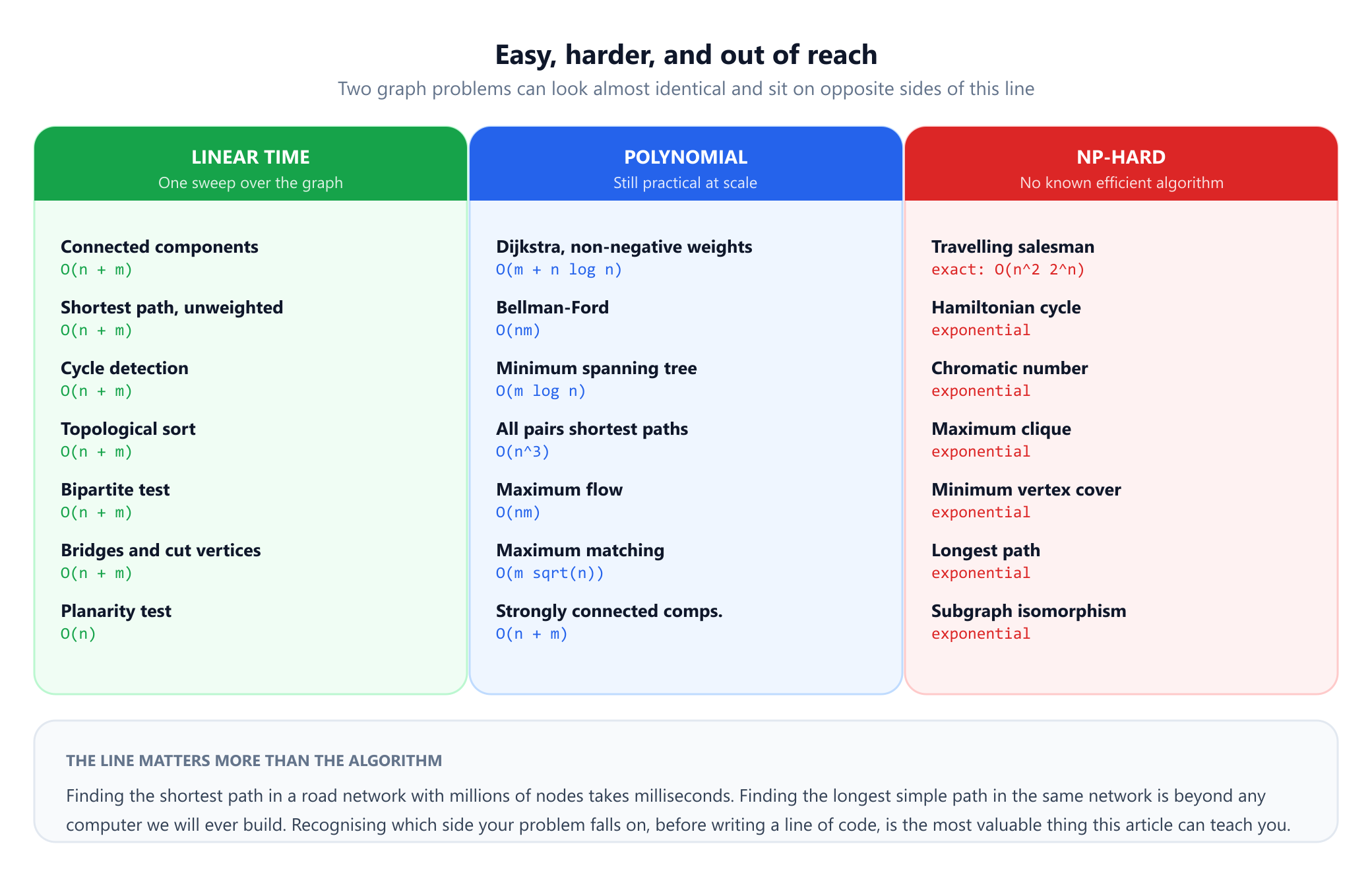
The formal statement is that a large family of graph problems is NP-complete, a notion introduced by Cook in 1971 and given its first substantial catalogue by Richard Karp in 1972, whose famous list of 21 problems is dominated by graph problems: clique, vertex cover, Hamiltonian circuit, chromatic number, feedback arc set and more. No polynomial time algorithm is known for any of them, and one for any one of them would give one for all of them. Nobody expects that to happen.
The practical consequence is not despair, it is a change of question. When a problem lands in the right hand column you stop asking for the optimum and choose among four honest strategies:
- Accept an approximation. For metric TSP, Christofides' 1976 algorithm guarantees a tour at most 1.5 times the optimum in polynomial time.
- Use a heuristic and measure it. Local search such as 2-opt or simulated annealing regularly lands within a couple of per cent of optimal on thousands of cities, with no guarantee at all.
- Exploit the structure of your instances. Hard in general does not mean hard for you: colouring is easy on chordal graphs, many problems are easy on trees and on graphs of small treewidth, and road networks have geometry that specialised routing algorithms exploit ruthlessly.
- Solve smaller instances exactly. Integer programming solvers routinely prove optimality for TSP instances with thousands of cities. Exponential does not mean impossible, it means the ceiling arrives quickly.
One caution: "NP-hard" describes worst cases as the input grows, not a verdict on your particular problem. A fuller treatment of the cost of each algorithm is in graph algorithms and complexity.
14. Where graphs actually show up
The claim that graph theory is everywhere is easy to make and worth substantiating. Here is where the material in this article is doing work right now, on the device you are reading this on.
Navigation. Every routing app models the road network as a weighted directed graph, junctions as vertices and road segments as arcs weighted by expected travel time. The query is a shortest path and the algorithm is an engineered descendant of Dijkstra and A*, using precomputed hierarchies so a continental route touches a few thousand vertices instead of tens of millions. One-way streets are why the graph must be directed; live traffic is why the weights change by the minute.
Search and social platforms. The web is a directed graph of pages and links, and PageRank, described by Brin and Page in 1998, ranks a page by the probability that a random surfer following links ends up there, which is an eigenvector computation on the adjacency structure. On social platforms people are vertices and relationships are edges: Milgram's 1967 letter study produced the popular "six degrees", and a 2012 analysis of the whole Facebook graph put the average distance between two users at 4.74. Community detection, friend recommendation and influence estimation are all standard graph computations run at scale.
Software engineering. Build systems, package managers and spreadsheet engines maintain a DAG and topologically sort it. Version control history is a DAG of commits, and a merge is a question about common ancestors. Compilers build control flow graphs for optimisation and interference graphs for register allocation, where assigning registers is literally graph colouring, and dead code elimination is a reachability query. See graph theory in software engineering.
Logistics. Delivery routing is the vehicle routing problem, warehouse placement is facility location and supply chains are flow networks with capacities. Here the gap between a good and a poor algorithm is measured in fuel and payroll, and the field that studies it is operations research.
Science and machine learning. A molecule is a graph of atoms and bonds, and searching a chemical database is subgraph isomorphism. Genome assembly reconstructs a sequence by finding an Eulerian path in a de Bruijn graph, which is Euler's 1736 criterion earning its keep 280 years later. Spectral clustering partitions data using the eigenvectors of a graph Laplacian, and graph neural networks generalise convolution to irregular structures by passing messages along edges. Power grids and telecoms are analysed for bridges and cut vertices because that is where cascading failures begin. A wider survey is in applications of graph theory.
15. Mistakes beginners reliably make
These are the errors that show up over and over in student code, in interviews and in production bugs. Every one of them is cheap to avoid once you have seen it named.
- Losing isolated vertices. Building the graph from an edge list means any vertex with no edges never appears. The order n silently changes, averages are wrong, and a component count is short. Build the vertex set first.
- Marking visited too late in BFS. Mark a vertex when you push it onto the queue, not when you pop it. Marking on pop lets the same vertex enter the queue once per incident edge, which turns a linear algorithm into a memory problem.
- Running BFS on a weighted graph. BFS minimises the number of edges, not their total weight. On a graph where a two-edge route costs 100 and a five-edge route costs 5, BFS confidently returns the expensive one. Weighted graphs need Dijkstra.
- Running Dijkstra with negative weights. Dijkstra assumes that once a vertex is settled, no cheaper route to it can appear later. A negative edge breaks that assumption and the output is silently wrong rather than an error. Use Bellman-Ford.
- Counting path length in vertices. Length is the number of edges, so a path through five vertices has length 4. This is the source of a large share of off-by-one errors in shortest path code.
- Ignoring which family the graph belongs to. An algorithm that is correct on undirected graphs can be silently wrong on directed ones, and a result proved for simple graphs may fail on a multigraph. Check the family before reaching for the algorithm.
- Assuming the graph is connected. Real data arrives in pieces. Check the component count before trusting any distance, diameter or average.
- Recursing too deep in DFS. A recursive DFS on a path of a million vertices needs a million stack frames. Write the iterative version when the input can be large.
- Adding only one direction in an undirected graph. An undirected edge must appear in both adjacency lists. Omitting the second append produces a graph that looks right in a drawing and behaves like a digraph in every traversal.
- Believing the drawing. Two edges crossing in a picture means nothing. Only the sets matter, which is why "is this graph planar" is a real question and not something you settle by squinting at a diagram.
- Assuming n - 1 edges means tree. It does only together with connectedness, or with acyclicity. A triangle plus an isolated vertex has 4 vertices and 3 edges and is not a tree.
16. Where to go next
The useful next step is to build a graph and run something on it rather than read more definitions. Type the running example into the interactive visualizer, run breadth first search from A and watch the layers fill in, then run depth first search from the same vertex and compare the order. Ninety seconds of that does what no amount of prose does.
After that, the natural sequence is the order of this article: vocabulary, traversal, weighted shortest paths, spanning trees, then the harder problems. The graph theory study roadmap lays out that path with a schedule and the structured lessons follow it interactively. For technical interviews, the graph theory for coding interviews guide covers the patterns that actually appear, alongside the algorithms cheat sheet.
For textbooks: West's Introduction to Graph Theory is the standard undergraduate course in book form, Diestel's Graph Theory is the graduate reference and the source of the definition in section 2, and the graph chapters of Cormen, Leiserson, Rivest and Stein remain the clearest treatment of the implementations. A fuller comparison, including courses and video series, is in the best resources to learn graph theory.
17. Glossary
Every term used above, in one place.
| Term | Meaning |
|---|---|
| Vertex (node) | An element of V. The theory assumes nothing about what it is. |
| Edge | A pair of vertices, {u, v} when undirected, (u, v) when directed. |
| Arc | A directed edge, with a tail and a head. |
| Order, size | The number of vertices n, and the number of edges m. |
| Adjacent | Two vertices joined by an edge. |
| Incident | The relation between an edge and one of its endpoints. |
| Degree | deg(v), the number of edge ends at v. A loop counts twice. |
| Neighbourhood | N(v), the set of vertices adjacent to v. |
| Simple graph | No loops and no parallel edges. |
| Multigraph | Parallel edges allowed; a pseudograph also allows loops. |
| Walk, trail, path | Any route; a route with no repeated edge; a route with no repeated vertex. |
| Cycle | A closed path of length at least 3 in a simple graph. |
| Length, distance | Edges in a route; the length of a shortest path, written d(u, v). |
| Connected, component | Every vertex reachable from every other; a maximal such piece. |
| Bridge, cut vertex | An edge, or a vertex, whose removal increases the component count. |
| Tree, forest | A connected acyclic graph; a disjoint union of trees. |
| Spanning tree | A tree subgraph containing every vertex of the graph. |
| Bipartite | Vertices split in two, with every edge crossing between the parts. |
| Complete graph | Kn, every pair joined, with n(n-1)/2 edges. |
| DAG | A directed graph with no directed cycle. |
| Planar | Drawable in the plane with no edges crossing. |
| Isomorphic | Identical up to renaming the vertices, so the same graph. |
| Sparse, dense | m close to n, against m close to n2. |
18. Frequently asked questions
What is graph theory in simple terms?
Graph theory is the study of connections. A graph is a set of objects, called vertices, together with a record of which pairs of them are joined, called edges. Nothing else is assumed, so the vertices can be cities, people, web pages or tasks. Because a great many practical questions depend only on which things are connected to which, one body of results and algorithms answers all of them at once.
What maths do I need before learning graph theory?
Much less than most people expect. Basic set notation, the idea of a function, and enough comfort with proofs to follow a counting argument are sufficient for a first course, and no calculus is needed anywhere. Linear algebra becomes useful if you go on to spectral methods, and probability if you go on to random graphs, but everything in this article needs arithmetic and careful reading only.
What is the difference between a graph and a tree?
A tree is a graph, specifically one that is connected and contains no cycles. Every tree is a graph, and most graphs are not trees. The useful properties follow from those two conditions: a tree on n vertices has exactly n-1 edges, there is exactly one path between any two vertices, and removing any edge disconnects it. Those constraints are why problems that are hard on general graphs are often easy on trees.
What is the difference between BFS and DFS?
Only the structure that holds the discovered vertices. Breadth first search uses a queue and explores layer by layer, so the first time it reaches a vertex it has used the fewest possible edges, which makes it the correct tool for shortest paths on unweighted graphs. Depth first search uses a stack, or recursion, and follows one branch as deep as it can before backtracking, which makes it the tool for structural questions such as cycle detection, topological ordering and finding bridges. Both visit every vertex once and both run in O(n + m) time.
Where is graph theory used in real life?
Route planning in navigation apps, PageRank in web search, friend and product recommendation on social platforms, dependency resolution in build systems and package managers, register allocation in compilers, genome assembly in bioinformatics, delivery routing in logistics, fraud detection in payment networks, and message passing in graph neural networks. Each one is a standard graph problem applied to a specific network.
Is graph theory important for coding interviews?
Yes. Graph questions are a reliable part of technical interviews at most large software companies, and the majority of them reduce to breadth first or depth first search with bookkeeping attached: grid traversal, counting islands, course scheduling by topological sort, cycle detection, and shortest paths on unweighted graphs. Fluency in the two traversals, plus the habit of building an adjacency list from whatever input format is given, covers most of what is actually asked.
Why can computers not solve the travelling salesman problem?
They can, for small instances, and they can get very close on large ones. What they cannot do is solve it exactly and quickly in every case, because the number of distinct tours through n cities is (n-1)!/2, which for just 20 cities is already more than 60 quadrillion. The problem is NP-hard, so no algorithm is known that escapes that growth in the worst case. In practice, exact solvers handle instances with thousands of cities, and heuristics such as 2-opt or simulated annealing land within a few per cent of optimal on much larger ones.
How long does it take to learn graph theory?
The foundations covered here, the definitions, both traversals and the standard problems, take most people two to four weeks of regular study. Being able to implement the classic algorithms from memory takes a couple of months of practice. The subject itself is open ended and still has active research, but the working knowledge that covers interviews and most engineering use is a small and finite body of material.
19. References
The definitions, theorems, dates and complexity bounds above come from these sources, listed in chronological order.
- Euler, L. (1736). "Solutio problematis ad geometriam situs pertinentis." Commentarii Academiae Scientiarum Petropolitanae 8 (published 1741), 128 to 140. The Königsberg bridges paper.
- Euler, L. (1758). "Elementa doctrinae solidorum." Novi Commentarii Academiae Scientiarum Petropolitanae 4, 109 to 140. The polyhedron formula behind n - m + f = 2.
- Kirchhoff, G. (1847). "Über die Auflösung der Gleichungen, auf welche man bei der Untersuchung der linearen Verteilung galvanischer Ströme geführt wird." Annalen der Physik 148(12), 497 to 508.
- Hierholzer, C. (1873). "Über die Möglichkeit, einen Linienzug ohne Wiederholung und ohne Unterbrechung zu umfahren." Mathematische Annalen 6(1), 30 to 32.
- Sylvester, J. J. (1878). "Chemistry and Algebra." Nature 17, 284. The first modern use of the word "graph".
- Cayley, A. (1889). "A theorem on trees." Quarterly Journal of Pure and Applied Mathematics 23, 376 to 378.
- Kuratowski, K. (1930). "Sur le problème des courbes gauches en topologie." Fundamenta Mathematicae 15, 271 to 283.
- König, D. (1931). "Gráfok és mátrixok." Matematikai és Fizikai Lapok 38, 116 to 119.
- König, D. (1936). Theorie der endlichen und unendlichen Graphen. Leipzig: Akademische Verlagsgesellschaft.
- Ford, L. R. and Fulkerson, D. R. (1956). "Maximal flow through a network." Canadian Journal of Mathematics 8, 399 to 404.
- Kruskal, J. B. (1956). "On the shortest spanning subtree of a graph and the traveling salesman problem." Proceedings of the American Mathematical Society 7(1), 48 to 50.
- Prim, R. C. (1957). "Shortest connection networks and some generalizations." Bell System Technical Journal 36(6), 1389 to 1401.
- Dijkstra, E. W. (1959). "A note on two problems in connexion with graphs." Numerische Mathematik 1, 269 to 271.
- Floyd, R. W. (1962). "Algorithm 97: Shortest path." Communications of the ACM 5(6), 345.
- Held, M. and Karp, R. M. (1962). "A dynamic programming approach to sequencing problems." Journal of the Society for Industrial and Applied Mathematics 10(1), 196 to 210.
- Milgram, S. (1967). "The small world problem." Psychology Today 2(1), 60 to 67.
- Cook, S. A. (1971). "The complexity of theorem-proving procedures." Proceedings of the Third Annual ACM Symposium on Theory of Computing, 151 to 158.
- Karp, R. M. (1972). "Reducibility among combinatorial problems." In Complexity of Computer Computations, 85 to 103. New York: Plenum Press.
- Tarjan, R. (1972). "Depth-first search and linear graph algorithms." SIAM Journal on Computing 1(2), 146 to 160.
- Hopcroft, J. and Tarjan, R. (1974). "Efficient planarity testing." Journal of the ACM 21(4), 549 to 568.
- Christofides, N. (1976). Worst-case analysis of a new heuristic for the travelling salesman problem. Report 388, Carnegie Mellon University.
- Appel, K. and Haken, W. (1977). "Every planar map is four colorable." Illinois Journal of Mathematics 21(3). Part I, 429 to 490; Part II, with J. Koch, 491 to 567.
- Fredman, M. L. and Tarjan, R. E. (1987). "Fibonacci heaps and their uses in improved network optimization algorithms." Journal of the ACM 34(3), 596 to 615.
- Brin, S. and Page, L. (1998). "The anatomy of a large-scale hypertextual Web search engine." Computer Networks and ISDN Systems 30(1 to 7), 107 to 117.
- West, D. B. (2001). Introduction to Graph Theory, 2nd edition. Upper Saddle River: Prentice Hall.
- Bondy, J. A. and Murty, U. S. R. (2008). Graph Theory. Graduate Texts in Mathematics 244. London: Springer.
- Gonthier, G. (2008). "Formal proof: the four-color theorem." Notices of the American Mathematical Society 55(11), 1382 to 1393.
- Cormen, T. H., Leiserson, C. E., Rivest, R. L. and Stein, C. (2009). Introduction to Algorithms, 3rd edition. Cambridge, Massachusetts: MIT Press.
- Backstrom, L., Boldi, P., Rosa, M., Ugander, J. and Vigna, S. (2012). "Four degrees of separation." Proceedings of the 4th Annual ACM Web Science Conference, 33 to 42.
- Diestel, R. (2017). Graph Theory, 5th edition. Graduate Texts in Mathematics 173. Berlin: Springer. Source of the definition quoted in section 2.
Build the running example yourself
Seven vertices, eight edges, and every definition on this page becomes something you can point at. Drop them into the visualizer, run BFS and DFS from A, and watch the two orders diverge.
Open the visualizer