
Table of Contents
- 1. What it means for two graphs to be the same
- 2. A graph that looks the same and is not
- 3. Invariants: proving two graphs are different
- 4. How many different graphs are there?
- 5. Testing by search
- 6. Colour refinement and its blind spot
- 7. Automorphisms: a graph's own symmetries
- 8. Canonical forms: one name per shape
- 9. How hard is graph isomorphism?
- 10. Subgraph isomorphism is a different problem
- 11. Where isomorphism testing is used
- 12. Common mistakes
- 13. Glossary
- 14. Frequently asked questions
- 15. References
1. What it means for two graphs to be the same
Two graphs are isomorphic when they are the same graph with different names on the vertices. Formally, G and H are isomorphic, written G ≅ H, if there is a bijection f from the vertices of G to the vertices of H such that u and v are adjacent in G exactly when f(u) and f(v) are adjacent in H. Such an f is an isomorphism. Both directions matter: edges must go to edges, and non-edges must go to non-edges.
Isomorphism ignores everything that is not structure. The names of the vertices do not count, and neither does the drawing: where the vertices sit on the page, how long the edges are, whether they cross. Two pictures that look nothing alike can show the same graph, and that is exactly what makes the question interesting. The guide to vertices and edges introduces the idea in one sentence; this article is about deciding it.
The running example is the triangular prism from the guide to planar graphs, called G here, and a second graph H drawn as a hexagon with three chords:
G = {AB, BC, CA, DE, EF, FD, AD, BE, CF}          two triangles and three rungs
H = {12, 23, 34, 45, 56, 61, 13, 25, 46}          hexagon 1..6 plus chords 13, 25, 46

f:  A→1   B→2   C→3   D→6   E→5   F→4
Check any edge of G and its image is an edge of H: AD goes to 16, DF goes to 64, BE goes to 25. Both graphs have nine edges and f maps the nine onto the nine, so it also sends non-edges to non-edges. G and H are the same graph. Being isomorphic is an equivalence relation, so graphs fall into isomorphism classes, which are what people usually mean by "the shapes" of graphs with a given number of vertices.
2. A graph that looks the same and is not
Now take a third graph K: the same hexagon, but with the three long diameters 14, 25 and 36 as chords. It has 6 vertices and 9 edges, every vertex has degree 3, and it is drawn in the same style as H. It is not isomorphic to G.
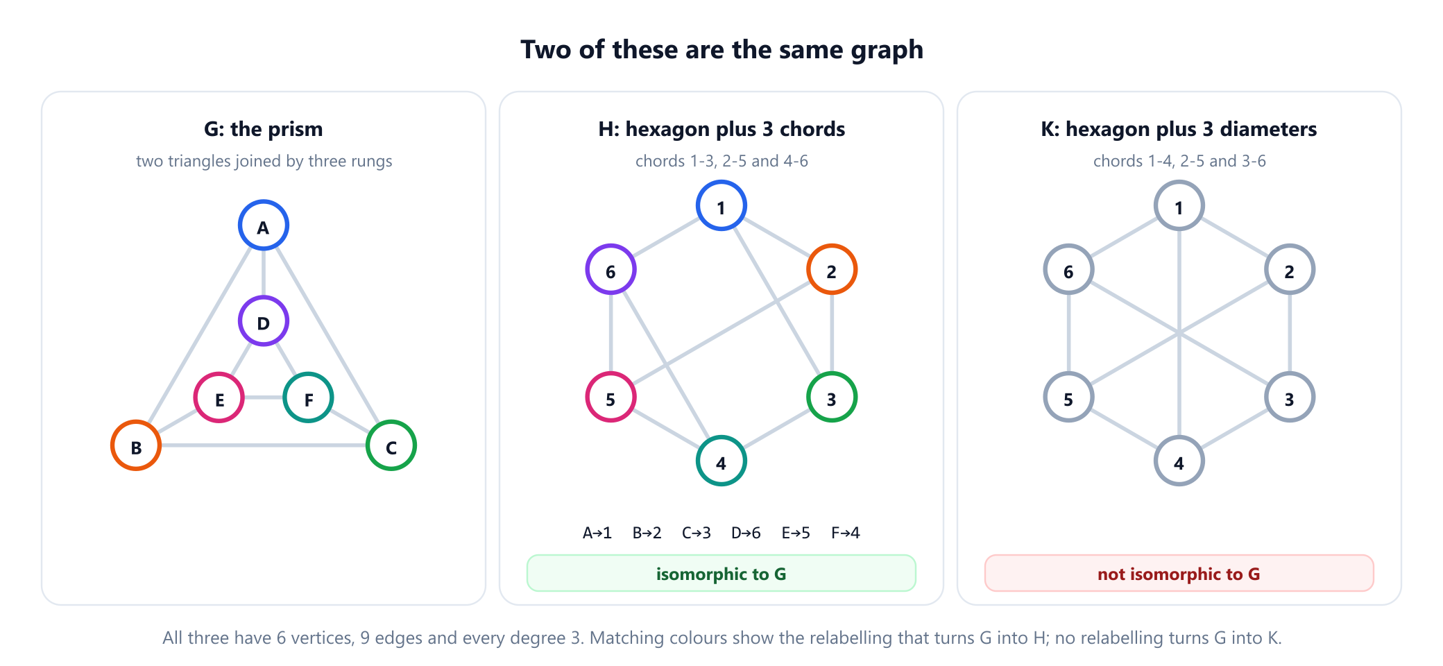
The quickest proof looks for triangles. G has two, ABC and DEF, and an isomorphism must send triangles to triangles. K has none: its vertices split into odd and even, and every edge joins an odd vertex to an even one, so K is bipartite and contains no cycle of odd length, as the guide to bipartite graphs explains. In fact K is the complete bipartite graph K3,3, the same graph that makes the three utilities puzzle impossible. Two graphs that agree on every obvious count can still be different, and much of the subject is about finding the count that tells them apart.
3. Invariants: proving two graphs are different
A graph invariant is any quantity that isomorphic graphs always share: the number of vertices and edges, the degree sequence, the number of triangles, whether the graph is connected or bipartite, its girth, its chromatic number, the eigenvalues of its adjacency matrix, and many more. Invariants work in one direction only.
If two graphs differ in any invariant, they are not isomorphic. If they agree on every invariant you computed, you have learned nothing certain.
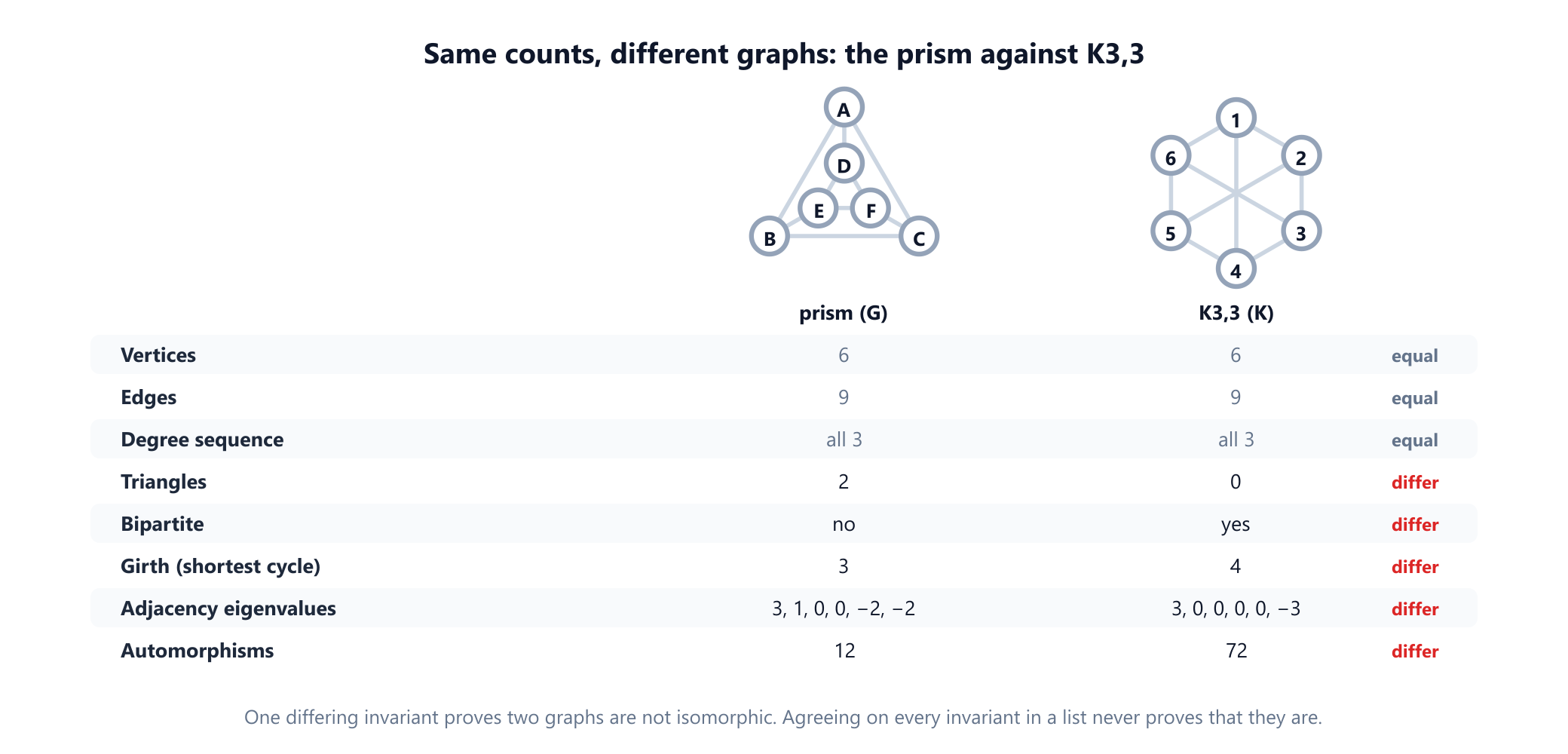
Every simple invariant has blind spots. The degree sequence misses the difference between the prism and K3,3. Even the full list of eigenvalues, which looks like a fingerprint, is not one: the star K1,4 and the 4-cycle plus an isolated vertex both have eigenvalues 2, 0, 0, 0, −2 and are clearly different graphs, the smallest such cospectral pair, credited to Collatz and Sinogowitz in 1957. An invariant that separated every pair of non-isomorphic graphs and could be computed quickly would settle the whole problem, and none is known.
4. How many different graphs are there?
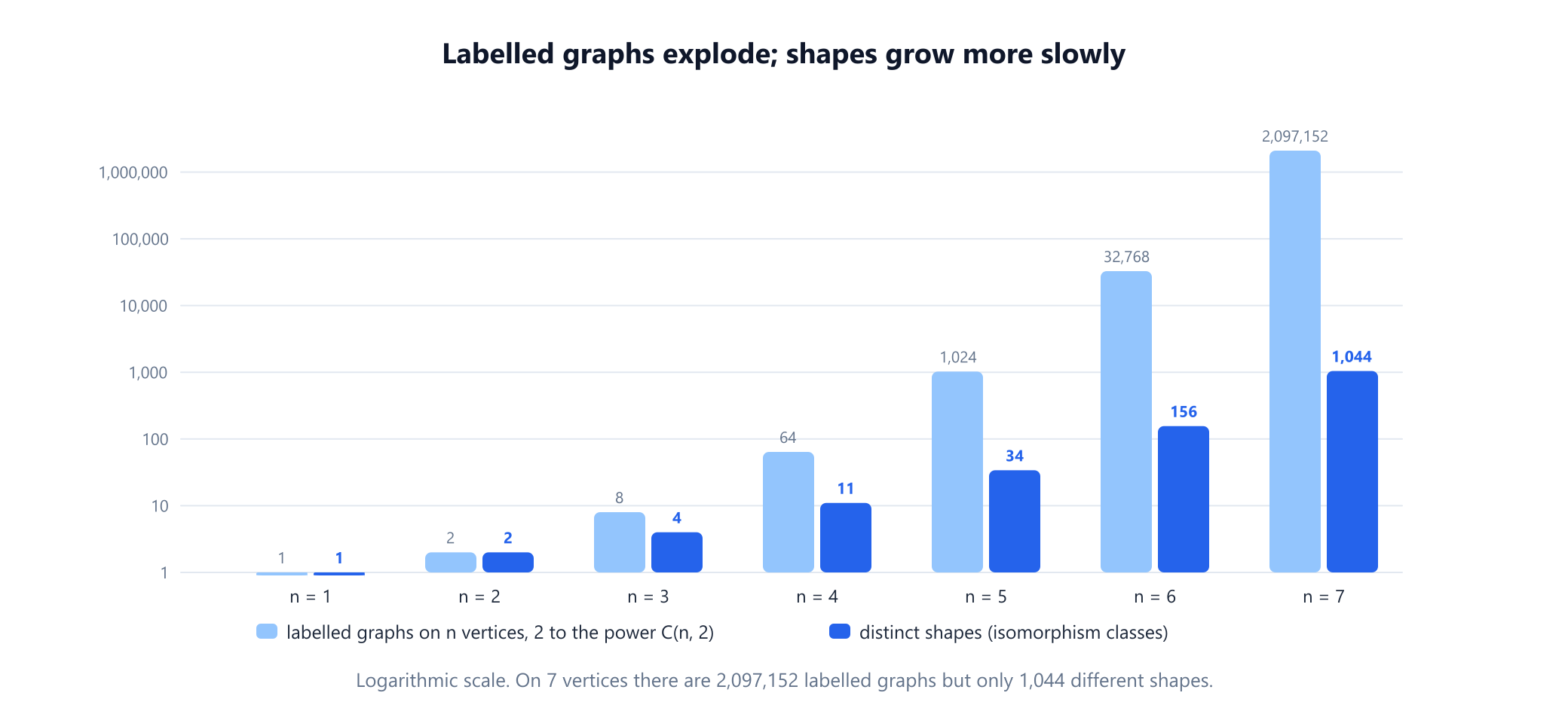
On n labelled vertices there are C(n, 2) possible edges, each present or absent, so 2C(n, 2) labelled graphs. Most of them are relabellings of each other. The number of genuinely different shapes, the isomorphism classes, grows far more slowly:
from itertools import combinations, permutations

def count_graphs(n):
    """Labelled graphs on n vertices, and how many distinct shapes they fall into."""
    pairs = list(combinations(range(n), 2))
    index = {p: i for i, p in enumerate(pairs)}
    seen, shapes = set(), 0
    for mask in range(1 << len(pairs)):
        if mask in seen:
            continue
        shapes += 1                           # a new isomorphism class: mark all its relabellings
        edges = [p for i, p in enumerate(pairs) if mask >> i & 1]
        for perm in permutations(range(n)):
            m = 0
            for u, v in edges:
                a, b = sorted((perm[u], perm[v]))
                m |= 1 << index[(a, b)]
            seen.add(m)
    return 1 << len(pairs), shapes

for n in range(1, 6):
    print(n, count_graphs(n))
# 1 (1, 1)
# 2 (2, 2)
# 3 (8, 4)
# 4 (64, 11)
# 5 (1024, 34)
The brute-force count stops at five vertices because it tries every relabelling of every graph. The sequence continues 156 for six vertices, 1,044 for seven and 12,346 for eight. There is no simple closed formula; the standard tool is Pólya's enumeration theory of 1937, which counts objects up to symmetry. The gap between the two columns is the reason isomorphism testing matters at all: a program that lists graphs, molecules or circuits has to recognise when two of its outputs are the same object in disguise.
5. Testing by search
The definition suggests an algorithm: try every bijection and check each one. With n vertices there are n! bijections, 720 for the six-vertex example but about 2.4 × 10¹⁸ for twenty vertices, so the naive method is hopeless beyond toy sizes. Two ideas make search practical on small and medium graphs. First, reject immediately when a cheap invariant such as the degree sequence differs. Second, build the mapping one vertex at a time, only try images of the same degree, and backtrack the moment an edge or non-edge fails to match.
def graph(edges):
    adj = {}
    for e in edges:
        u, v = e.split('-')
        adj.setdefault(u, set()).add(v)
        adj.setdefault(v, set()).add(u)
    return adj

def isomorphisms(G, H):
    """Yield every bijection f: V(G) -> V(H) with uv an edge exactly when f(u)f(v) is."""
    if len(G) != len(H) or sorted(map(len, G.values())) != sorted(map(len, H.values())):
        return                                # a cheap invariant already says no
    order = sorted(G, key=lambda v: -len(G[v]))
    def extend(f, used):
        if len(f) == len(order):
            yield dict(f)
            return
        u = order[len(f)]
        for x in H:
            if x in used or len(H[x]) != len(G[u]):
                continue                      # degrees must match
            if all((w in G[u]) == (f[w] in H[x]) for w in f):
                f[u] = x                      # consistent with every vertex mapped so far
                yield from extend(f, used | {x})
                del f[u]
    yield from extend({}, set())

G = graph(['A-B', 'B-C', 'C-A', 'D-E', 'E-F', 'F-D', 'A-D', 'B-E', 'C-F'])   # the prism
H = graph(['1-2', '2-3', '3-4', '4-5', '5-6', '6-1', '1-3', '2-5', '4-6'])   # hexagon + 3 chords
K = graph(['1-2', '2-3', '3-4', '4-5', '5-6', '6-1', '1-4', '2-5', '3-6'])   # hexagon + 3 diameters

print(next(isomorphisms(G, H)))
# {'A': '1', 'B': '2', 'C': '3', 'D': '6', 'E': '5', 'F': '4'}
print(sum(1 for _ in isomorphisms(G, H)))     # as many as G has symmetries
# 12
print(next(isomorphisms(G, K), None))         # same degrees, no isomorphism
# None
The first line of output is the mapping from section 1. The second shows that there are exactly 12 different isomorphisms from G to H, and section 7 explains why that number is not an accident. The third confirms that no mapping from the prism to K3,3 exists, even though the degree check passed. The function was checked against networkx on 3,000 random pairs of graphs, half of them relabelled copies of each other, with every mapping it returned verified edge by edge. Backtracking is still exponential in the worst case: graphs where every vertex looks alike defeat the degree pruning, and that is where the next idea comes in.
6. Colour refinement and its blind spot
Colour refinement, also called the one-dimensional Weisfeiler–Leman algorithm after Weisfeiler and Leman's 1968 paper, gives every vertex a colour and keeps refining the colours using the neighbourhoods. Start with one colour for everyone. In each round, give two vertices the same new colour only if they had the same old colour and their neighbours carry the same multiset of old colours. Stop when no colour class splits. Run it on two graphs together: if the final colour counts differ, the graphs are not isomorphic.
from collections import Counter

def colour_refinement(adj, rounds=None):
    """1-WL: repeatedly recolour each vertex by its colour plus the multiset of its neighbours' colours."""
    colour = {v: 0 for v in adj}
    for _ in range(rounds or len(adj)):
        signature = {v: (colour[v], tuple(sorted(colour[w] for w in adj[v]))) for v in adj}
        palette = {s: i for i, s in enumerate(sorted(set(signature.values())))}
        new = {v: palette[signature[v]] for v in adj}
        if len(set(new.values())) == len(set(colour.values())):
            break                             # stable: no colour class split
        colour = new
    return colour

def joint(G, H):
    """True if refinement cannot tell G and H apart. Refine them together so colours match."""
    union = {('g', v): {('g', w) for w in G[v]} for v in G}
    union.update({('h', v): {('h', w) for w in H[v]} for v in H})
    c = colour_refinement(union)
    return (sorted(Counter(c[k] for k in union if k[0] == 'g').items()) ==
            sorted(Counter(c[k] for k in union if k[0] == 'h').items()))

def graph(edges):
    adj = {}
    for e in edges:
        u, v = e.split('-')
        adj.setdefault(u, set()).add(v)
        adj.setdefault(v, set()).add(u)
    return adj

T1 = graph(['a-b', 'b-c', 'c-d', 'b-e', 'e-f'])       # centre b, legs of length 2, 2 and 1
T2 = graph(['a-b', 'b-c', 'c-d', 'd-e', 'b-f'])       # centre b, legs of length 3, 1 and 1
prism = graph(['A-B', 'B-C', 'C-A', 'D-E', 'E-F', 'F-D', 'A-D', 'B-E', 'C-F'])
k33 = graph(['1-2', '2-3', '3-4', '4-5', '5-6', '6-1', '1-4', '2-5', '3-6'])

print(joint(T1, T2))      # same degree sequence, but refinement tells them apart
# False
print(joint(prism, k33))  # both 3-regular: refinement cannot tell them apart
# True
The two trees in the example have the same degree sequence, (3, 2, 2, 1, 1, 1), so the degree check cannot separate them. Refinement can: after a few rounds a leaf next to the centre and a leaf at the end of a long leg get different colours, and the colour counts of the two trees no longer match. Refinement is strong in general. Babai, Erdős and Selkow showed in 1980 that a simple degree-based refinement identifies almost all graphs, so on a random graph isomorphism is easy.
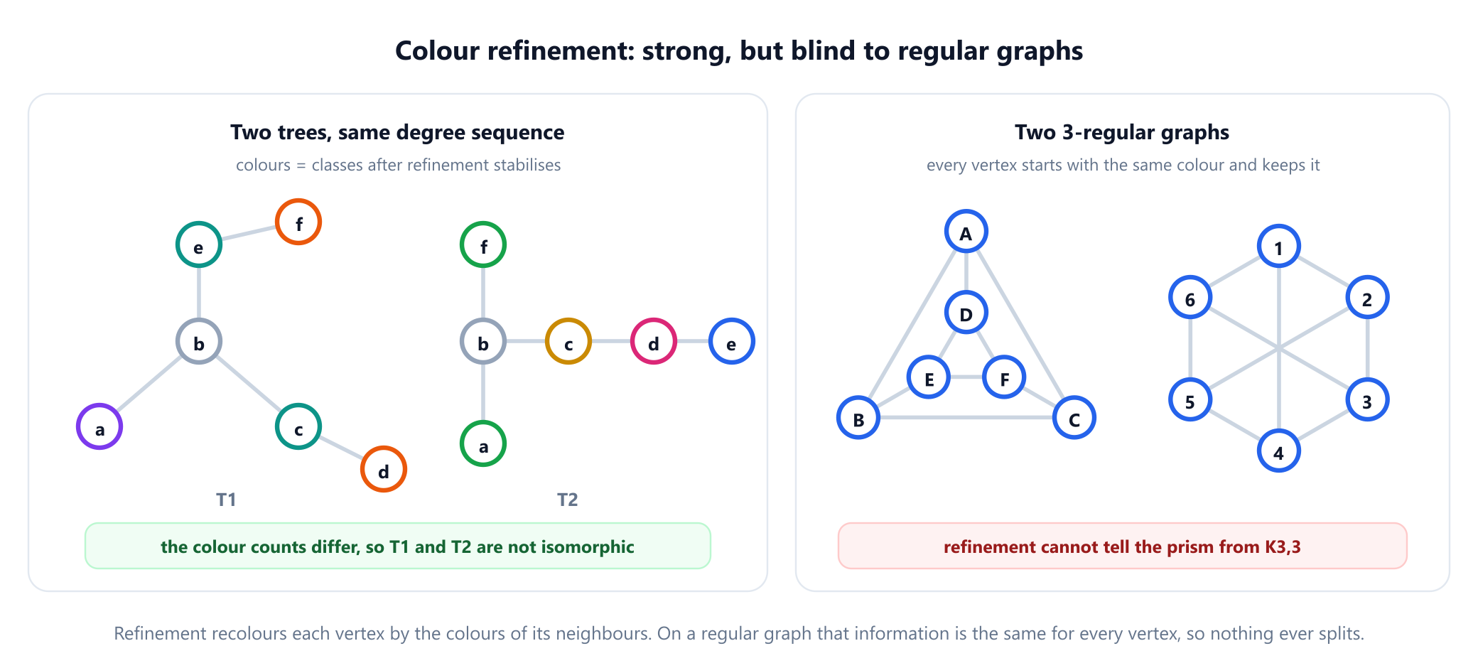
The blind spot is regularity. In a k-regular graph every vertex starts with the same colour and has k neighbours of that colour, so the first round changes nothing and the algorithm stops at once. Any two regular graphs with the same number of vertices and the same degree look identical to it, which is why the prism and K3,3 pass this test together. The same limit reaches into machine learning: Xu and colleagues proved in 2019 that message-passing graph neural networks can distinguish two graphs only if colour refinement can, which is why the guide to graph neural networks treats the Weisfeiler–Leman test as their yardstick. Stronger versions refine colours of pairs or triples of vertices instead of single vertices; they see more but cost more.
7. Automorphisms: a graph's own symmetries
An isomorphism from a graph to itself is an automorphism, a symmetry of the graph. The automorphisms of a graph form a group, and its size measures how symmetric the graph is. The prism has 12: rotate or reflect the two triangles together, which gives 6 symmetries, and optionally swap the two triangles. K3,3 has 72, since each side can be permuted in 6 ways and the two sides can be swapped, and the Petersen graph has 120.
This explains the 12 in section 5. If f is one isomorphism from G to H, then every other one is f combined with an automorphism of G, so isomorphic graphs always have exactly as many isomorphisms between them as either has automorphisms. A search that wants only one answer wastes time exploring symmetric copies of the same mapping, and the best practical algorithms use the automorphisms they discover to prune the search.
Two classical results show how far symmetry can go in each direction. Frucht proved in 1939 that every finite group is the automorphism group of some graph, so symmetry can take any form at all. And Erdős and Rényi proved in 1963 that almost all graphs are asymmetric, with no automorphism except the identity. Small graphs are deceptive here: no graph with between two and five vertices is asymmetric, the smallest asymmetric graphs have six vertices and there are eight of them, and among the 1,044 graphs on seven vertices only 152 are asymmetric. The "almost all" takes over only as n grows.
8. Canonical forms: one name per shape
Comparing graphs in pairs does not scale when a database holds millions of them. The alternative is a canonical form: a relabelling rule that sends every graph to one fixed representative of its isomorphism class, so that two graphs are isomorphic exactly when their canonical forms are identical. Once each graph has a canonical form, isomorphism becomes equality of strings, and a database can index, hash and deduplicate graphs like any other key.
The simplest canonical form takes, over all n! relabellings, the one whose adjacency matrix reads smallest as a string of bits. That is correct and far too slow. Practical tools compute canonical forms with individualisation and refinement: run colour refinement, and when it gets stuck on a class of look-alike vertices, single one of them out with a new colour and refine again, exploring a search tree of such choices and pruning it with the automorphisms found along the way. McKay's program nauty, described in 1981, and Traces, presented with nauty by McKay and Piperno in 2014, work this way and handle graphs with many thousands of vertices in practice.
9. How hard is graph isomorphism?
Graph isomorphism has an unusual place in complexity theory. It is in NP, because a proposed mapping can be checked in polynomial time. It is not known to be solvable in polynomial time. And it is unlikely to be NP-complete: Boppana, Håstad and Zachos showed in 1987 that if it were, the polynomial hierarchy would collapse to its second level, which most researchers consider implausible. It is one of very few natural problems believed to sit strictly between the easy and the NP-complete.
The best general algorithm is Babai's. He announced it in November 2015 and published it at STOC in 2016: graph isomorphism can be decided in quasipolynomial time, exp((log n)O(1)), which is not polynomial but enormously better than exponential. In January 2017 Helfgott found an error in one step, Babai withdrew the quasipolynomial claim, and within days he announced a repair, which Helfgott confirmed. For special classes much more is known:
- Trees can be tested in linear time with the algorithm of Aho, Hopcroft and Ullman, which builds a canonical code for each tree from its leaves up, the technique discussed in trees in graph theory.
- Planar graphs can be tested in linear time, as Hopcroft and Wong showed in 1974.
- Graphs of bounded degree can be tested in polynomial time, a result of Luks from 1982 that became a building block of Babai's algorithm.
10. Subgraph isomorphism is a different problem
A close relative asks whether one graph appears inside another: is there a subgraph of H that is isomorphic to G? This subgraph isomorphism problem is much harder. Cook's 1971 paper, the one that founded the theory of NP-completeness, already showed it to be as hard as satisfiability, NP-complete in today's terms. It contains the clique problem as a special case: asking whether a graph contains Kk is asking whether Kk is a subgraph of it.
The two problems are easy to confuse because they share a name and an algorithmic style. Practical subgraph matchers such as Ullmann's 1976 algorithm and VF2 by Cordella and colleagues in 2004 use the same backtracking-with-pruning idea as section 5, but they are searching for a pattern, not a perfect match, and no quasipolynomial bound is expected for them. When someone says a problem is "a graph isomorphism problem", it is worth asking which of the two they mean.
11. Where isomorphism testing is used
- Chemistry. A molecule's bonds form a graph, and chemical databases use canonical forms to store each structure once and to look a compound up instantly. Graph isomorphism is necessary but not sufficient for chemical identity: stereoisomers share the same bond graph and differ in their arrangement in space.
- Circuit verification. Checking that a chip layout implements its schematic, known as layout versus schematic, includes matching the transistor network extracted from the layout against the intended one.
- Enumeration and databases. Generating all graphs, all molecules or all designs of a given size requires discarding duplicates, which is a canonical-form computation for every candidate.
- Machine learning on graphs. The Weisfeiler–Leman connection in section 6 is used both to measure what graph neural networks can express and as a fast baseline for comparing graphs.
- Symmetry in optimisation. Automorphisms of a problem's structure mean many equivalent solutions; detecting them lets a solver skip the copies.
12. Common mistakes
| Mistake | Why it is wrong | Fix |
|---|---|---|
| "Same degree sequence, so isomorphic" | The prism and K3,3 are both 3-regular on 6 vertices | Use invariants only to prove graphs different; find a mapping to prove them the same |
| Checking only that edges map to edges | A map can send edges to edges and still add new ones in the image | Require edges and non-edges both to be preserved, or check equal edge counts |
| Judging by the drawing | H and K are drawn alike and differ; G and H are drawn differently and agree | Ignore positions; compare structure |
| Treating equal spectra as proof | K1,4 and C4 plus a vertex are cospectral and different | Treat the spectrum as an invariant, not a certificate |
| Relying on colour refinement for regular graphs | It cannot distinguish any two regular graphs of the same size and degree | Use individualisation and refinement, as nauty does |
| Confusing isomorphism with subgraph isomorphism | The first is quasipolynomial; the second is NP-complete | Check whether you need a perfect match or a pattern inside a larger graph |
| Calling graph isomorphism NP-complete | It is in NP but is not believed to be NP-complete | Say "not known to be in P", and mention Babai's quasipolynomial algorithm |
13. Glossary
| Term | Meaning |
|---|---|
| Isomorphism | A bijection between vertex sets that preserves adjacency and non-adjacency |
Isomorphic, G ≅ H | Having an isomorphism between them; the same graph up to names |
| Isomorphism class | All graphs isomorphic to a given one; a "shape" of graph |
| Graph invariant | A quantity that isomorphic graphs always share |
| Cospectral graphs | Graphs with the same adjacency eigenvalues |
| Colour refinement, 1-WL | Iterative recolouring of vertices by their neighbours' colours |
| Automorphism | An isomorphism from a graph to itself; a symmetry |
| Asymmetric graph | A graph whose only automorphism is the identity |
| Canonical form | A fixed representative of an isomorphism class, computed from any member |
| Individualisation and refinement | Singling out a vertex, refining again, and searching over such choices |
| Quasipolynomial time | Running time exp((log n)O(1)) |
| Subgraph isomorphism | Deciding whether one graph appears inside another; NP-complete |
14. Frequently asked questions
What does it mean for two graphs to be isomorphic?
Two graphs are isomorphic when there is a one-to-one correspondence between their vertices that preserves adjacency: two vertices are joined in the first graph exactly when their images are joined in the second. Isomorphic graphs are the same graph with different vertex names, however differently they are drawn.
How do you tell whether two graphs are isomorphic?
First compare invariants such as the number of vertices and edges, the degree sequence and the number of triangles. Any difference proves the graphs are not isomorphic. If all of them agree, search for a mapping by backtracking, trying only vertices of matching degree, or use a tool such as nauty that computes canonical forms. Agreement on invariants alone is never a proof.
What is a graph invariant?
A graph invariant is a property that isomorphic graphs always share, such as the number of edges, the degree sequence, the number of triangles, bipartiteness, girth or the eigenvalues of the adjacency matrix. A differing invariant proves two graphs are different. No invariant that is known to be fast to compute separates every pair of non-isomorphic graphs.
Is graph isomorphism NP-complete?
Graph isomorphism is in NP, but it is not known to be NP-complete and is widely believed not to be: if it were, the polynomial hierarchy would collapse. It is also not known to be solvable in polynomial time. Babai showed in 2016 that it can be solved in quasipolynomial time, which is far faster than exponential.
What is the Weisfeiler-Leman test?
The one-dimensional Weisfeiler-Leman test, or colour refinement, repeatedly recolours every vertex by its own colour and the multiset of its neighbours' colours. If two graphs end with different colour counts, they are not isomorphic. It identifies almost all graphs but cannot distinguish any two regular graphs with the same number of vertices and the same degree.
What is the difference between graph isomorphism and subgraph isomorphism?
Graph isomorphism asks whether two graphs are the same. Subgraph isomorphism asks whether one graph appears inside another as a subgraph. The second is NP-complete and contains the clique problem as a special case, while graph isomorphism can be solved in quasipolynomial time.
15. References
The definitions, theorems and attributions above come from these sources, listed in chronological order.
- Pólya, G. (1937). "Kombinatorische Anzahlbestimmungen für Gruppen, Graphen und chemische Verbindungen." Acta Mathematica 68, 145 to 254. Counting objects up to symmetry.
- Frucht, R. (1939). "Herstellung von Graphen mit vorgegebener abstrakter Gruppe." Compositio Mathematica 6, 239 to 250.
- Collatz, L. and Sinogowitz, U. (1957). "Spektren endlicher Grafen." Abhandlungen aus dem Mathematischen Seminar der Universität Hamburg 21, 63 to 77. Cospectral graphs.
- Erdős, P. and Rényi, A. (1963). "Asymmetric Graphs." Acta Mathematica Academiae Scientiarum Hungaricae 14, 295 to 315.
- Weisfeiler, B. and Leman, A. (1968). "The Reduction of a Graph to Canonical Form and the Algebra Which Appears Therein." Nauchno-Technicheskaya Informatsia, Series 2, no. 9, 12 to 16.
- Cook, S. A. (1971). "The Complexity of Theorem-Proving Procedures." Proceedings of the 3rd Annual ACM Symposium on Theory of Computing, 151 to 158. Subgraph isomorphism as hard as satisfiability.
- Aho, A. V., Hopcroft, J. E. and Ullman, J. D. (1974). The Design and Analysis of Computer Algorithms. Reading, Massachusetts: Addison-Wesley. Linear-time tree isomorphism.
- Hopcroft, J. E. and Wong, J. K. (1974). "Linear Time Algorithm for Isomorphism of Planar Graphs (Preliminary Report)." Proceedings of the 6th Annual ACM Symposium on Theory of Computing, 172 to 184.
- Ullmann, J. R. (1976). "An Algorithm for Subgraph Isomorphism." Journal of the ACM 23(1), 31 to 42.
- Babai, L., Erdős, P. and Selkow, S. M. (1980). "Random Graph Isomorphism." SIAM Journal on Computing 9(3), 628 to 635.
- McKay, B. D. (1981). "Practical Graph Isomorphism." Congressus Numerantium 30, 45 to 87.
- Luks, E. M. (1982). "Isomorphism of Graphs of Bounded Valence Can Be Tested in Polynomial Time." Journal of Computer and System Sciences 25(1), 42 to 65.
- Boppana, R. B., Håstad, J. and Zachos, S. (1987). "Does co-NP Have Short Interactive Proofs?" Information Processing Letters 25(2), 127 to 132.
- Cordella, L. P., Foggia, P., Sansone, C. and Vento, M. (2004). "A (Sub)Graph Isomorphism Algorithm for Matching Large Graphs." IEEE Transactions on Pattern Analysis and Machine Intelligence 26(10), 1367 to 1372.
- McKay, B. D. and Piperno, A. (2014). "Practical Graph Isomorphism, II." Journal of Symbolic Computation 60, 94 to 112.
- Babai, L. (2016). "Graph Isomorphism in Quasipolynomial Time." Proceedings of the 48th Annual ACM Symposium on Theory of Computing, 684 to 697.
- Diestel, R. (2017). Graph Theory, 5th edition. Graduate Texts in Mathematics 173. Berlin: Springer.
- Xu, K., Hu, W., Leskovec, J. and Jegelka, S. (2019). "How Powerful are Graph Neural Networks?" International Conference on Learning Representations.
Build the impostor yourself
Draw the prism and K3,3 in the visualizer and run the bipartite check on both. One splits into two sides, the other finds an odd cycle at once: the invariant that tells them apart.
Open the visualizer