
Table of Contents
Graph traversal is the foundational mechanism of almost all graph theory algorithms. It is the systematic process of visiting, checking, analyzing, and often updating each vertex (node) in a graph. Whether you are finding the shortest route on Google Maps, recommending friends on a social network, crawling the internet for a search engine, or solving a complex puzzle algorithmically, you are utilizing graph traversal.
At the heart of this domain lie two legendary algorithms: Breadth-First Search (BFS) and Depth-First Search (DFS). While both guarantee that every reachable node in a connected component will be visited exactly once, the order and strategy by which they visit nodes lead to drastically different applications, time/space complexities, and behavioral patterns.
In this comprehensive guide, we will dissect both algorithms, analyze their data structures, review implementation code, compare their complexities, and finally look at real-world scenarios to help you confidently answer the ultimate question: "When should I use BFS, and when should I use DFS?"
1. Deep Dive into Breadth-First Search (BFS)
Breadth-First Search explores the graph in concentric "waves." It starts at a chosen root node (or arbitrary starting node) and visits all immediate neighbors first. Only after completely exhausting all nodes at a distance of exactly 1 edge away does it move on to nodes at distance 2, and so forth.
The Water Drop Analogy: Think of BFS like a drop of water creating ripples in a still pond. The ripple expands outward uniformly in all directions. It does not shoot off in one straight line; it covers area equally by radius.
The Mechanics of BFS
To ensure that nodes are visited in this strictly layer-by-layer fashion, BFS relies on a Queue (First-In, First-Out, or FIFO) data structure to keep track of which nodes to visit next.
The standard BFS algorithm follows these steps:
- Initialize a Queue and a boolean array (or Hash Set) to keep track of
visitednodes. - Enqueue the starting node and immediately mark it as
visited. - Begin a loop that continues as long as the Queue is not empty.
- Dequeue the front node. This is your current node. Process it as needed.
- Iterate over every adjacent neighbor of this current node.
- If a neighbor has not been visited, mark it as
visitedand enqueue it. - Repeat until the queue is empty.
BFS Implementation Example
Below is a clean implementation of BFS in Python using an adjacency list representation and the highly efficient collections.deque.
from collections import deque

def breadth_first_search(graph, start_node):
    # Initialize a queue and a set to keep track of visited nodes
    queue = deque([start_node])
    visited = {start_node}

    # Store the traversal order
    traversal_order = []

    while queue:
        # Dequeue a vertex from the front of the queue
        current_node = queue.popleft()
        traversal_order.append(current_node)

        # Get all adjacent vertices of the dequeued vertex
        for neighbor in graph[current_node]:
            if neighbor not in visited:
                # Mark as visited IMMEDIATELY before enqueuing
                # to prevent duplicate entries in the queue
                visited.add(neighbor)
                queue.append(neighbor)

    return traversal_order

# Example Graph (Adjacency List)
graph = {
    'A': ['B', 'C'], 'B': ['A', 'D', 'E'], 'C': ['A', 'F'], 'D': ['B'], 'E': ['B', 'F'], 'F': ['C', 'E']
}

print(breadth_first_search(graph, 'A'))
# Output: ['A', 'B', 'C', 'D', 'E', 'F']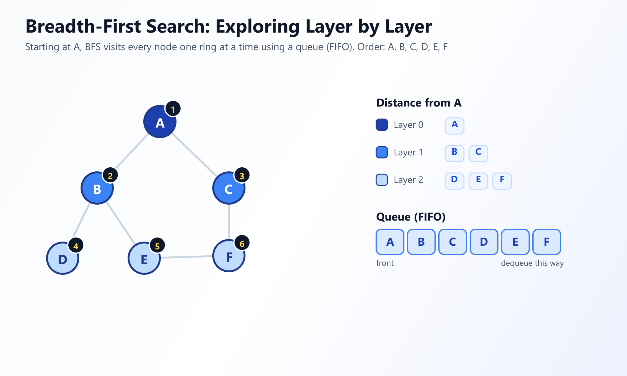
Stop Reading, Start Visualizing
Reading code is good, but watching the algorithm execute in real-time builds true intuition. Watch how the Queue manages the BFS wave on our platform.
Launch Interactive BFS Visualizer2. Deep Dive into Depth-First Search (DFS)
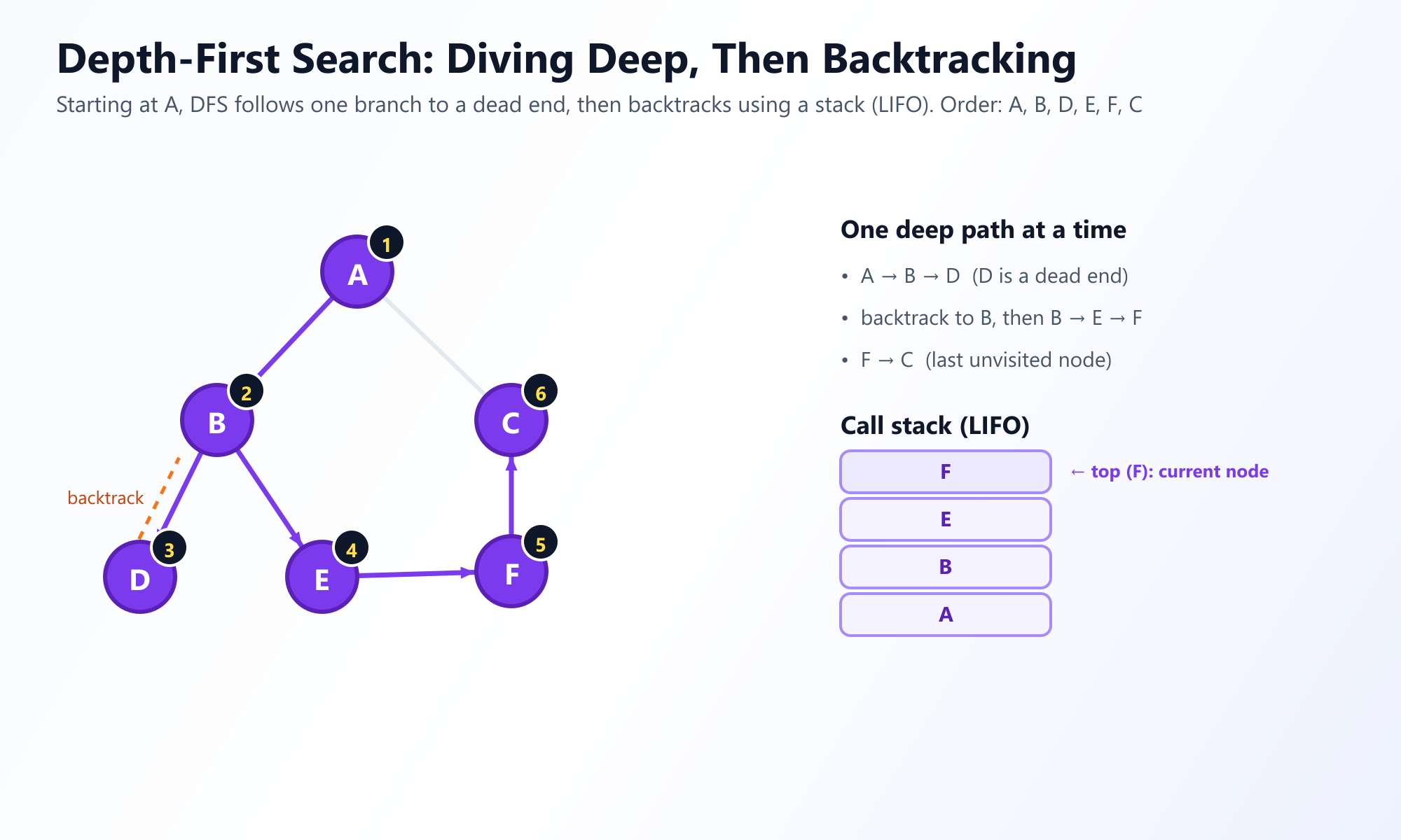
Depth-First Search takes a drastically different, more aggressive approach. Instead of exploring broadly, it explores deeply. It starts at a root node and explores as far as possible along a singular branch until it hits a "dead end" (a node with no unvisited neighbors). Once stuck, it retreats or backtracks up the path just enough to find a new, unexplored branch to dive down.
The Maze Runner Analogy: Think of DFS like navigating a physical labyrinth. You place your hand on the right wall and keep walking forward. You keep taking turns until you hit a dead end, at which point you turn around, walk back to the last intersection, and take the unexplored path.
The Mechanics of DFS
Because DFS needs to remember where it came from so it can backtrack, it utilizes a Stack (Last-In, First-Out, or LIFO) data structure. Most commonly, developers implement DFS recursively, elegantly utilizing the CPU's native call stack rather than creating a manual stack object.
The standard Recursive DFS algorithm follows these steps:
- Start at the current node and immediately mark it as
visited. - Process the node (e.g., print its value).
- Iterate over all its adjacent neighbors.
- If a neighbor has not been visited, recursively call the DFS function on that neighbor.
- When the loop finishes (no unvisited neighbors remain), the function returns, automatically backtracking to the previous caller on the stack.
DFS Implementation Example
Below is an elegant recursive implementation of DFS in Python.
def depth_first_search_recursive(graph, current_node, visited=None, traversal_order=None):
    # Initialize collections on the first call
    if visited is None:
        visited = set()
    if traversal_order is None:
        traversal_order = []

    # Mark the current node as visited and record it
    visited.add(current_node)
    traversal_order.append(current_node)

    # Recursively visit all unvisited neighbors
    for neighbor in graph[current_node]:
        if neighbor not in visited:
            depth_first_search_recursive(graph, neighbor, visited, traversal_order)

    return traversal_order

# Example Graph (Adjacency List)
graph = {
    'A': ['B', 'C'], 'B': ['A', 'D', 'E'], 'C': ['A', 'F'], 'D': ['B'], 'E': ['B', 'F'], 'F': ['C', 'E']
}

print(depth_first_search_recursive(graph, 'A'))
# Output: ['A', 'B', 'D', 'E', 'F', 'C']
Notice the difference in output compared to BFS. DFS aggressively pursued the path A to B to D before backtracking.
Visualize the Backtracking Magic
Recursive call stacks can be hard to map in your head. Watch how DFS dives deep and visually backtracks along the edges when it gets stuck.
Launch Interactive DFS Visualizer3. BFS vs. DFS: The Ultimate Comparison
In technical interviews and real-world system design, choosing the wrong traversal algorithm can lead to catastrophic memory exhaustion or highly inefficient execution times. Let's break down the technical differences.

| Metric | Breadth-First Search (BFS) | Depth-First Search (DFS) |
|---|---|---|
| Data Structure | Queue (FIFO) - Iterative approach | Stack (LIFO) - Often Recursive approach |
| Time Complexity | O(V + E)Must visit every Vertex (V) and check every Edge (E). |
O(V + E)Also visits every Vertex and explores every Edge. |
| Space Complexity | O(W) where W is the maximum width of the graph.Can be O(V) in worst-case dense graphs. |
O(H) where H is the maximum depth/height of the graph.Can be O(V) if the graph is a single long line. |
| Shortest Path Guaranty | Yes. For unweighted graphs, BFS is guaranteed to find the shortest path. | No. DFS might find a highly convoluted, massive path before finding the short, direct one. |
| Memory Footprint | High if the tree/graph is very wide (e.g., social network). The queue must hold all nodes in the current level. | High if the tree/graph is very deep. The call stack must hold all ancestors of the current node. |
| Optimality | Optimal for finding targets close to the source. | Optimal for finding targets far from the source or exploring all possibilities. |
Understanding the Space Complexity Trade-off
While both algorithms have a time complexity of O(V + E), their space complexities drastically differ depending on the topology of the graph.
- Wide Graphs: If a graph has a massive branching factor (e.g., an HTML DOM tree, or a Twitter follower graph), the BFS Queue will balloon in size because it must store an entire "level" of the graph at once. In these scenarios, DFS is highly memory efficient.
- Deep Graphs: If a graph is extremely deep (e.g., a massive blockchain or a deep decision tree), DFS might exceed the maximum recursion depth or consume too much stack memory. In these scenarios, BFS might be preferable, though iterative deepening DFS is often the actual solution used in production.
4. Real-World Applications: When to use which?
The choice between BFS and DFS usually comes down to what you are trying to extract from the graph structure.
Use Breadth-First Search when:
- Finding the Shortest Path (Unweighted Graphs): Because BFS explores level by level, the first time it encounters the target node, it has definitively taken the fewest number of edges to get there. GPS routing algorithms often use variations of BFS (like Dijkstra's) for this reason.
- Target is likely close to the source: If you are searching a family tree for an immediate cousin, BFS will find them instantly. DFS might explore an entirely different branch of the family back to the 16th century before checking the cousin.
- Peer-to-Peer Networks: Protocols like BitTorrent use BFS to find neighbor nodes. "Find all peers 1 hop away, then 2 hops away."
- Web Crawlers: Search engines like Google initially used BFS to crawl the web. They want to index the most prominent links on the main page before diving deeply into obscure, nested sub-pages.
- Social Network "Degrees of Separation": Features like LinkedIn's "2nd-degree connection" rely entirely on BFS limits.
Use Depth-First Search when:
- Checking for Cycles: DFS is uniquely equipped to find back-edges (edges pointing back to an ancestor). If a back-edge exists, the graph has a cycle. This is critical for preventing infinite loops in routers and detecting deadlocks in operating systems.
- Topological Sorting: In build systems (like Make, Webpack, or npm), tasks have dependencies. DFS is used to linearly order these tasks so that every task is executed only after its dependencies are met.
- Memory is heavily constrained (and the graph is wide): As discussed, DFS only needs to store the path from the root to the current node, making it incredibly memory-efficient for wide, massive graphs like game-state trees (e.g., Chess engines).
- Solving Puzzles and Mazes: DFS is the algorithm of choice for solving Sudoku, N-Queens, or generating/solving physical mazes. It aggressively explores a possible solution, and if it fails, it simply backtracks and tries the next configuration.
- Finding Strongly Connected Components: Algorithms like Tarjan's or Kosaraju's rely heavily on DFS to group nodes into strongly connected clusters.
5. Advanced Variations
In modern computer science, raw BFS and raw DFS are often augmented to handle massive scales.
- Bidirectional BFS: Instead of running BFS from the source to the target, you run two simultaneous BFS waves - one from the source and one from the target. When the waves intersect, you've found the shortest path. This drastically reduces the search space area.
- Iterative Deepening DFS (IDDFS): This combines the space-efficiency of DFS with the shortest-path guarantee of BFS. It runs a DFS but sets a strict depth limit. If the target isn't found, it increments the depth limit and starts over. It's heavily used in AI and game tree analysis.
Conclusion
Breadth-First Search and Depth-First Search are the undisputed cornerstones of graph theory. BFS is your expansive, level-by-level wave, perfect for shortest paths and broad network analysis. DFS is your aggressive, memory-efficient maze runner, perfect for cycle detection, topological sorting, and deep puzzle solving.
Mastering both algorithms is non-negotiable for passing technical interviews at top tech companies and for designing robust, scalable software architectures.
Frequently Asked Questions
When should I choose BFS over DFS?
Choose Breadth-First Search (BFS) when you need to find the shortest path in an unweighted graph, or when you are searching for a target node known to be close to the starting point.
When is DFS more advantageous than BFS?
Depth-First Search (DFS) is better for exploring all possibilities (e.g., maze solving), topological sorting, cycle detection, or when you have memory constraints, as DFS uses less memory on deep graphs.
How do the data structures used by BFS and DFS differ?
BFS uses a Queue (First-In, First-Out) to explore level by level. DFS uses a Stack (Last-In, First-Out), which is often implemented implicitly using recursion.