The Vehicle Routing Problem (VRP) Explained

Mohammed Islam Hadjoudj

Expert Operations Research Engineer

1. What is the Vehicle Routing Problem?

The Vehicle Routing Problem (VRP) is a combinatorial optimization and integer programming problem that asks: "What is the optimal set of routes for a fleet of vehicles to traverse in order to deliver to a given set of customers?"

Introduced in 1959 by George Dantzig and John Ramser, the VRP is a central problem in the fields of transportation, distribution, and logistics. The goal is typically to minimize the total route cost (which could mean minimizing distance, time, fuel, or the number of vehicles used) while ensuring that every customer is visited exactly once.

In a standard VRP:

• There is a central Depot where all vehicles start and end their journeys.
• There is a Fleet of vehicles, all assumed to be identical in the base problem.
• There is a set of Customers, each located at a specific node on a graph.

2. VRP vs. TSP: Understanding the Difference

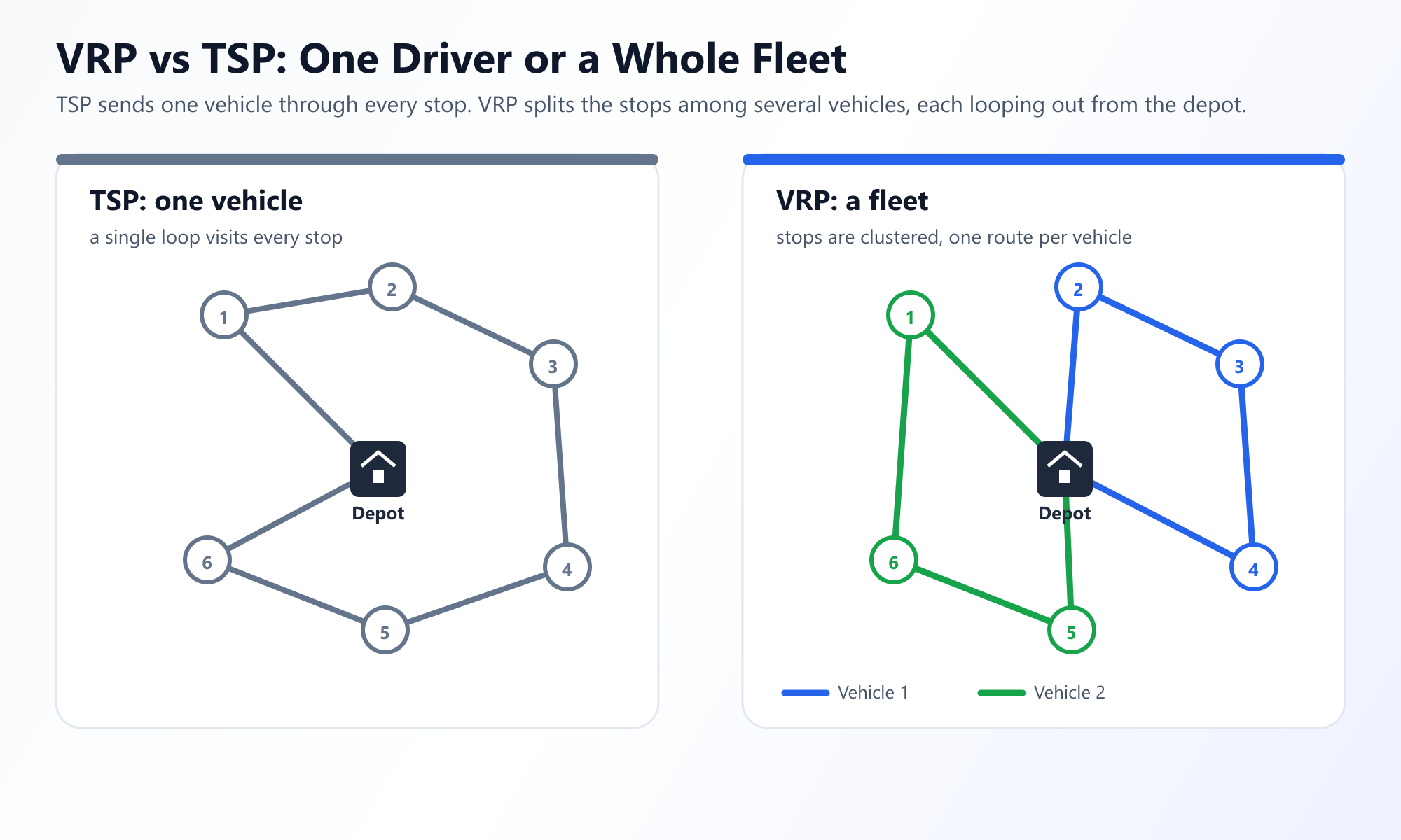
If you are familiar with graph theory, the VRP sounds suspiciously like the Traveling Salesperson Problem (TSP). In fact, the VRP is a generalization of the TSP.

The core difference is the number of actors:

• TSP: You have one salesperson who must visit every city and return home.
• VRP: You have multiple vehicles. You must first cluster the cities (assigning a specific group of cities to Vehicle A, another group to Vehicle B), and then solve a mini-TSP for each vehicle.

Because the TSP is already NP-Hard (computationally intractable for exact solutions at large scales), the VRP is also NP-Hard, but significantly more complex due to the added clustering dimension.

3. Common Variations of VRP

The basic VRP assumes infinite vehicle capacity and no time constraints. In the real world, a FedEx truck cannot carry infinite packages. This has led to the creation of several highly practical variations of the VRP.

Capacitated Vehicle Routing Problem (CVRP)

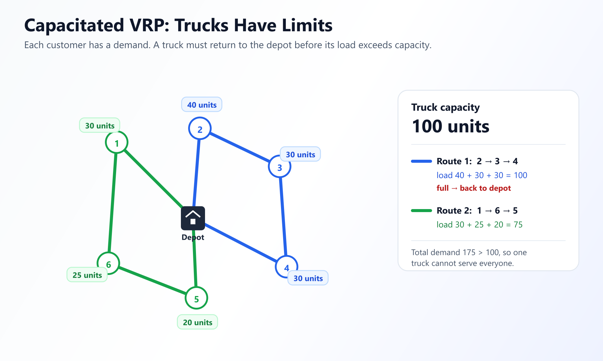
In the CVRP, every vehicle has a maximum carrying capacity (e.g., a truck can hold 500 lbs), and every customer has a specific demand (e.g., Customer A needs 50 lbs of goods). A vehicle's route must end, and it must return to the depot, before the sum of the demands on its route exceeds its capacity. This is the most common variation studied in operations research.

Vehicle Routing Problem with Time Windows (VRPTW)

In the VRPTW, customers require deliveries within specific time frames. For example, a restaurant might need its ingredients delivered between 8:00 AM and 10:00 AM. If a truck arrives at 7:30 AM, it must wait. If it arrives at 10:15 AM, the delivery fails. This adds severe timing constraints to the routing logic.

Other Notable Variations

• VRPPD (Pickup and Delivery): Vehicles don't just drop off goods; they pick them up from customers and deliver them to other customers (like Uber or DoorDash).
• MDVRP (Multi-Depot VRP): A company has multiple warehouses (depots). The algorithm must decide not only the routes but also which depot serves which customer.
• SDVRP (Split Delivery VRP): A customer's demand is so large that it can be split and fulfilled by multiple different vehicles.

4. How is the VRP Solved?

Because the VRP is NP-Hard, calculating the absolute perfect set of routes for hundreds of customers is practically impossible. Instead, logistics companies rely on a two-phase approach to find "near-optimal" routes very quickly.

Phase 1: Cluster First, Route Second

The most intuitive human approach is also used by algorithms. First, group the customers into clusters based on geographical proximity and vehicle capacity. Once you have a cluster of customers assigned to a specific truck, you treat that cluster as a standalone Traveling Salesperson Problem and solve for the shortest path.

Phase 2: Metaheuristics

Once an initial set of routes is established, algorithms attempt to continuously improve them. These are known as metaheuristics.

• Simulated Annealing: The algorithm occasionally accepts "worse" routes in the short term to escape local optimums, slowly "cooling down" to settle on a globally efficient route.
• Genetic Algorithms: Takes multiple good routing solutions, "breeds" them together by swapping sections of routes, and keeps the "fittest" (shortest) offspring.
• Tabu Search: An aggressive local search that keeps a memory (a tabu list) of recently evaluated routes to prevent the algorithm from getting stuck in infinite loops.

5. The Clarke and Wright Savings Algorithm

If you want to write a VRP solver, the best place to start is the Clarke and Wright Savings Algorithm, developed in 1964. It remains one of the most famous and widely implemented heuristics for the Capacitated VRP (CVRP).

The logic is based on the concept of "savings."

1. Start with the worst case: Imagine you have 10 customers. You send 10 separate trucks out from the depot. Truck 1 goes to Customer 1 and returns. Truck 2 goes to Customer 2 and returns, etc.
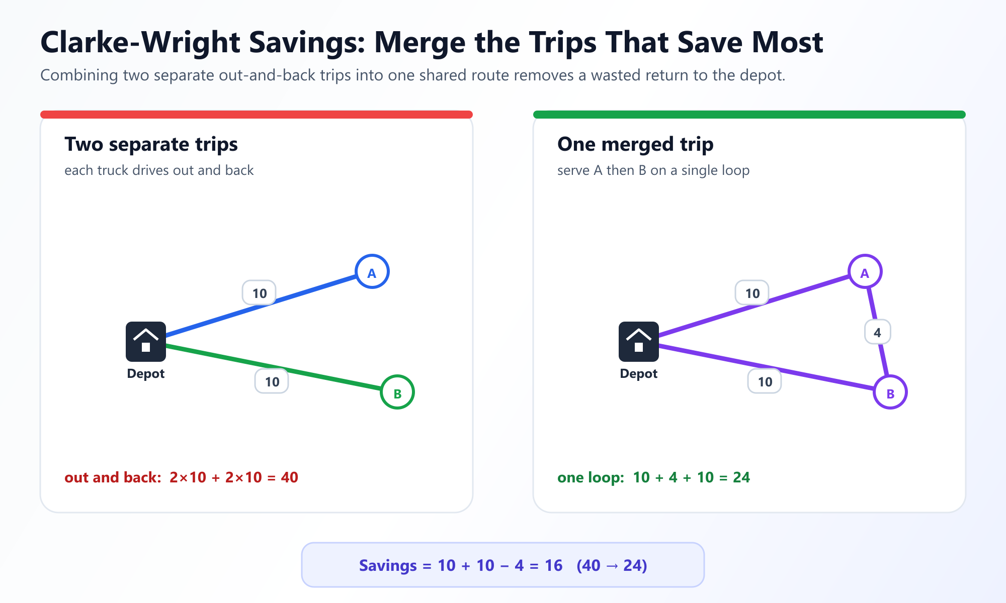
2. Calculate Savings: If you combine the routes (Depot -> Customer 1 -> Customer 2 -> Depot), how much distance do you save compared to sending two separate trucks? You calculate this "savings" value for every possible pair of customers.
3. Sort and Merge: You sort the pairs by the highest savings. You then aggressively merge routes together, starting with the biggest savings, provided that the combined route does not exceed the vehicle's maximum capacity.

This algorithm runs in O(n^2 log n) time and produces highly efficient routes almost instantly, serving as the baseline upon which metaheuristics can improve.

6. Real-World Applications

A 5% improvement in VRP optimization translates to millions of dollars in savings for major corporations.

• Package Delivery (UPS/FedEx): UPS famously uses an optimization system called ORION (On-Road Integrated Optimization and Navigation). By heavily penalizing left-hand turns in their VRP calculations (which waste gas while waiting at traffic lights), UPS saves over 10 million gallons of fuel a year.
• Ridesharing (Uber/Lyft): UberPool is a massive, real-time Dynamic VRP with Pickup and Delivery. The algorithm must continuously re-cluster and re-route vehicles as new ride requests appear dynamically.
• Waste Management: Garbage trucks must route through every street in a city (a subset of VRP known as the Capacitated Arc Routing Problem), ensuring the trucks return to the dump before hitting their weight limits.