
Table of Contents
- 1. Every vertex, exactly once
- 2. From the Icosian game to the Petersen graph
- 3. Proving that no cycle exists
- 4. Degree conditions that guarantee a cycle
- 5. Planar graphs: Tait's conjecture and Tutte's answer
- 6. Finding a Hamiltonian path by search
- 7. Dynamic programming over subsets
- 8. How hard is the problem?
- 9. Families that always have one
- 10. Random graphs: when do Hamiltonian cycles appear?
- 11. Where Hamiltonian paths are used
- 12. Common mistakes
- 13. Glossary
- 14. Frequently asked questions
- 15. References
1. Every vertex, exactly once
A Hamiltonian path is a path that visits every vertex of a graph exactly once. A Hamiltonian cycle does the same and then returns to its starting vertex along one more edge. A graph with a Hamiltonian cycle is called Hamiltonian, and a graph with a Hamiltonian path is sometimes called traceable. Every Hamiltonian graph is traceable, since deleting one edge of a Hamiltonian cycle leaves a Hamiltonian path, but the reverse fails, as the examples below show.
The question sounds like a close relative of the one Euler answered in 1736, and the guide to Eulerian paths tells that story. An Eulerian trail uses every edge once; a Hamiltonian path visits every vertex once. The difference in difficulty is enormous. Euler's question is settled by counting odd degrees, which takes linear time. For Hamilton's question no comparable test is known, and none is expected to exist.
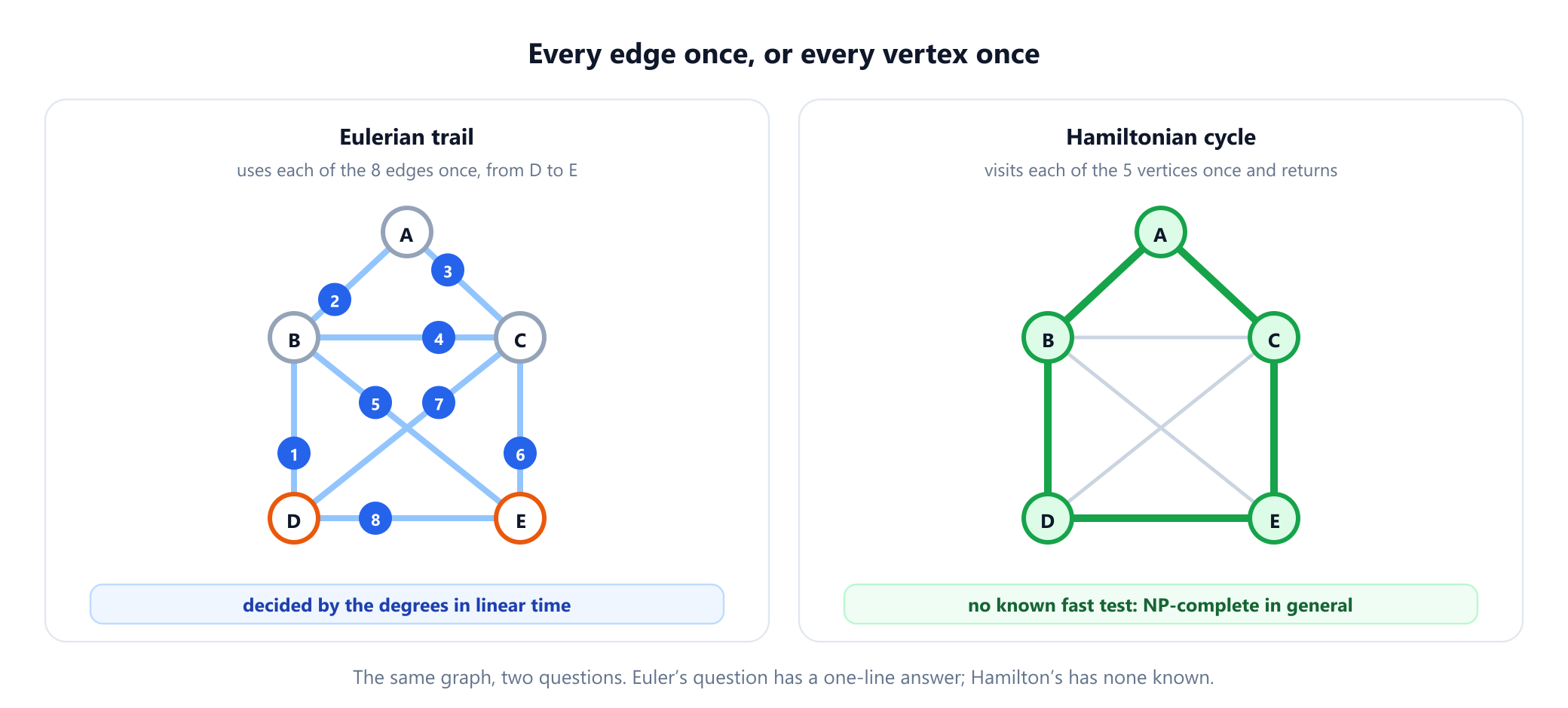
In the house-shaped graph above, vertex A has degree 2, B and C have degree 4, and D and E have degree 3. Exactly two degrees are odd, so an Eulerian trail runs from D to E, and the degrees alone prove it. The Hamiltonian cycle A, B, D, E, C also exists, but the only general way to know is to find it.
2. From the Icosian game to the Petersen graph
The name comes from William Rowan Hamilton, who in 1857 presented the Icosian game: a board drawn as a dodecahedron, the solid with 12 pentagonal faces and 20 corners, on which the player had to visit all 20 corners and return to the start along the edges. Hamilton sold the rights for 25 pounds to the London firm of John Jaques and Son, which put the game on sale in 1859. The question itself is older: Thomas Kirkman had asked in a paper published in 1856 which polyhedra have a circuit through all of their corners.
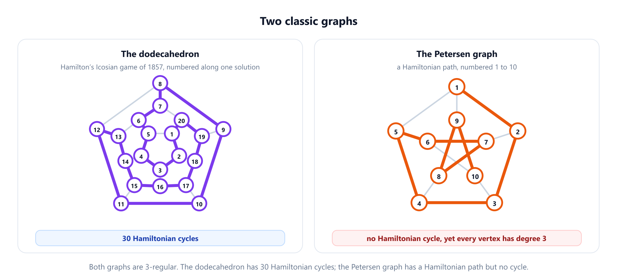
The dodecahedron has exactly 30 Hamiltonian cycles, counting each cycle once regardless of its direction and starting corner. The Petersen graph, which Julius Petersen described in 1898, is the classic contrast. It has 10 vertices and 15 edges, every vertex has degree 3, it is connected and has no cut vertex, and yet it has no Hamiltonian cycle. It does have a Hamiltonian path. Stranger still, deleting any one of its vertices leaves a graph that does have a Hamiltonian cycle, a property called hypohamiltonian. Every simple test that suggests a graph should be Hamiltonian is satisfied by the Petersen graph, which is why it appears as a counterexample throughout graph theory.
3. Proving that no cycle exists
The running example is a museum with 9 rooms, A to I, and 14 doors between them. A visitor wants to see every room exactly once, and ideally to finish where they started:
doors = {AB, AC, BC, FG, FH, GH, AD, BD, DF, DI, CE, EH, EI, EG}      9 rooms, 14 doors

deg:   A 3   B 3   C 3   D 4   E 4   F 3   G 3   H 3   I 2
A Hamiltonian path exists: A, B, C, E, G, H, F, D, I visits every room once. A Hamiltonian cycle does not, and the reason can be seen in a picture. Close rooms D and E, and the rest of the museum falls into three separate pieces: {A, B, C}, {F, G, H} and the single room I.
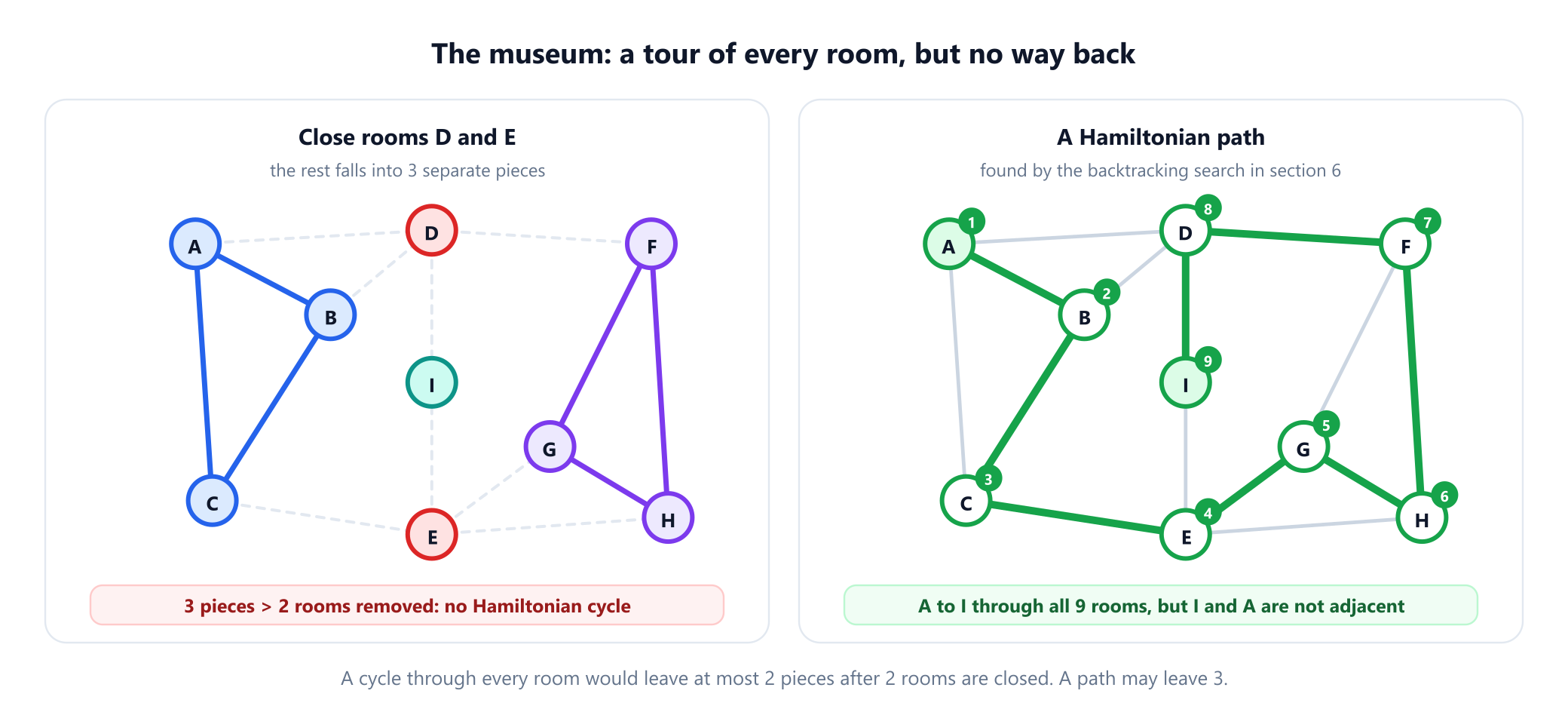
The argument works for any graph. Delete k vertices from a cycle and it breaks into at most k arcs, so if a graph has a Hamiltonian cycle, deleting any k of its vertices leaves at most k connected pieces. A path breaks into at most k + 1 pieces, so a traceable graph leaves at most k + 1. The museum has a set of 2 rooms whose removal leaves 3 pieces, which is too many for a cycle but allowed for a path. Chvátal studied this measure in 1973 under the name toughness.
from itertools import combinations

def graph(edges):
    adj = {}
    for u, v in edges:
        adj.setdefault(u, set()).add(v)
        adj.setdefault(v, set()).add(u)
    return adj

def pieces(adj, removed):
    """Number of connected pieces left after deleting the vertices in removed."""
    seen, count = set(removed), 0
    for s in adj:
        if s in seen:
            continue
        count += 1
        stack = [s]
        seen.add(s)
        while stack:
            for w in adj[stack.pop()] - seen:
                seen.add(w)
                stack.append(w)
    return count

def cycle_obstruction(adj):
    """A set S whose removal leaves more than |S| pieces: proof that no Hamiltonian cycle exists."""
    for k in range(1, len(adj)):
        for S in combinations(sorted(adj), k):
            if pieces(adj, S) > k:
                return list(S), pieces(adj, S)
    return None

museum = graph(['AB', 'AC', 'BC', 'FG', 'FH', 'GH', 'AD', 'BD', 'DF', 'DI', 'CE', 'EH', 'EI', 'EG'])
print(cycle_obstruction(museum))
# (['D', 'E'], 3)
outer = [(i, (i + 1) % 5) for i in range(5)]
spokes = [(i, i + 5) for i in range(5)]
star = [(5 + i, 5 + (i + 2) % 5) for i in range(5)]
petersen = graph(outer + spokes + star)
print(cycle_obstruction(petersen))            # no certificate, yet no Hamiltonian cycle either
# None
The function tries every set of vertices, smallest first, and returns the first one that leaves too many pieces. On the museum it finds {D, E}, the only such set. On the Petersen graph it finds nothing, even though the Petersen graph has no Hamiltonian cycle. That is the limit of every condition of this kind: it can prove that a cycle is impossible, but its silence proves nothing.
Several special cases of the same idea are worth knowing by name:
- Cut vertices. A graph with a cut vertex, one whose removal disconnects it, has no Hamiltonian cycle. This is the case
k = 1. - Vertices of degree 1 or 2. A vertex of degree 1 can only be an end of a Hamiltonian path, never part of a cycle. A vertex of degree 2 forces both of its edges into any Hamiltonian cycle: in the museum, both of room
I's doors would have to be used. - Unbalanced bipartite graphs. A cycle in a bipartite graph alternates between the two sides, so a Hamiltonian cycle needs sides of equal size, and a Hamiltonian path needs sizes that differ by at most one. The complete bipartite graph
K2,3has a Hamiltonian path but no Hamiltonian cycle for this reason.
4. Degree conditions that guarantee a cycle
The opposite direction asks what forces a Hamiltonian cycle to exist. The most famous answers use degrees, and the guide to vertex degree treats the first of them in detail.
- Dirac's theorem (1952). A simple graph with
n ≥ 3vertices in which every vertex has degree at leastn / 2has a Hamiltonian cycle. - Ore's theorem (1960). It is enough that
deg(u) + deg(v) ≥ nfor every pair of verticesuandvthat are not adjacent. Dirac's condition is the special case where every degree is at leastn / 2. - The Bondy–Chvátal closure (1976). Repeatedly join any two non-adjacent vertices whose degrees add up to at least
n. The original graph is Hamiltonian exactly when the final graph, its closure, is Hamiltonian; if the closure is complete, the answer is yes. - The Chvátal–Erdős theorem (1972). If the connectivity of a graph, the fewest vertices whose removal disconnects it, is at least its independence number, the size of its largest independent set, then the graph is Hamiltonian. The guide to cliques and independent sets explains the second quantity.
All of these are sufficient conditions, not necessary ones. A cycle on 100 vertices is Hamiltonian, yet every vertex has degree 2, far below 50. The museum shows the other side: its largest degree is 4, below 9 / 2, so none of the degree conditions applies, which is consistent with its having no cycle. After one more door is opened, between G and I, the museum becomes Hamiltonian, and the degree conditions still say nothing. They describe graphs that are dense enough to be Hamiltonian for easy reasons; sparse graphs need other tools.
5. Planar graphs: Tait's conjecture and Tutte's answer
Hamiltonian cycles once looked like a route to the four colour theorem. In 1884 Peter Guthrie Tait conjectured that every 3-connected, 3-regular planar graph has a Hamiltonian cycle, which would have given an easy proof that four colours suffice for maps whose corners all meet three regions. The conjecture was false. William Tutte published a counterexample with 46 vertices in 1946, and Holton and McKay showed in 1988 that the smallest counterexamples have 38 vertices.
One more degree of connectivity is enough. Whitney proved in 1931 that every 4-connected planar triangulation is Hamiltonian, and Tutte extended this in 1956 to every 4-connected planar graph. These results are among the few that guarantee Hamiltonian cycles in sparse graphs, where the degree conditions of section 4 cannot apply.
6. Finding a Hamiltonian path by search
The direct method extends a path one vertex at a time. At each step it tries the unvisited neighbours of the last vertex in turn; when the path cannot be extended and some vertex is still unvisited, it backs up and tries the next choice. If the path ever covers every vertex, it is a Hamiltonian path, and if its two ends are adjacent, it also closes into a cycle.
def graph(edges):
    adj = {}
    for u, v in edges:
        adj.setdefault(u, set()).add(v)
        adj.setdefault(v, set()).add(u)
    return adj

def hamiltonian(adj, cycle=False):
    """Backtracking: extend a path one vertex at a time and undo it at a dead end."""
    n = len(adj)
    def extend(path, seen):
        if len(path) == n:
            return path if not cycle or path[0] in adj[path[-1]] else None
        for w in sorted(adj[path[-1]] - seen):
            found = extend(path + [w], seen | {w})
            if found:
                return found
        return None                           # every continuation failed: back up
    starts = [min(adj)] if cycle else sorted(adj)   # a cycle may start anywhere
    for s in starts:
        found = extend([s], {s})
        if found:
            return found
    return None

museum = graph(['AB', 'AC', 'BC', 'FG', 'FH', 'GH', 'AD', 'BD', 'DF', 'DI', 'CE', 'EH', 'EI', 'EG'])
print(hamiltonian(museum))                    # visit every room once
# ['A', 'B', 'C', 'E', 'G', 'H', 'F', 'D', 'I']
print(hamiltonian(museum, cycle=True))        # ... and come back to the start
# None
museum['G'].add('I'); museum['I'].add('G')    # open one more door
print(hamiltonian(museum, cycle=True))
# ['A', 'B', 'C', 'E', 'H', 'F', 'G', 'I', 'D']
The first line is the tour from section 3. The second confirms that no tour can return to its start, as the obstruction proved. The third shows that opening one more door, between G and I, makes a Hamiltonian cycle possible. When searching for a cycle the function starts from a single vertex, because a cycle passes through every vertex and can be read from any of them. The function was checked against brute force on 1,136 random graphs with up to 8 vertices.
Plain backtracking is exponential: in the worst case it explores a large share of the n! orderings of the vertices, and 20! is about 2.4 × 10¹⁸. Practical solvers add pruning. They abandon a branch as soon as the unvisited vertices are disconnected, or a vertex has too few unvisited neighbours left to be passed through, or a degree-2 vertex has its forced edges blocked. They also try the most constrained neighbour first, the same idea as Warnsdorff's rule for knight's tours in section 9.
7. Dynamic programming over subsets
A better worst case comes from a dynamic program found independently by Bellman and by Held and Karp in 1962, originally for the travelling salesperson problem. Fix a start vertex. For every subset S of vertices containing it and every vertex v in S, record how many paths start at the fixed vertex, visit exactly the vertices of S, and end at v. Each entry is built from smaller subsets, and the full set gives the Hamiltonian paths, which close into cycles when their last vertex is adjacent to the start.
from itertools import combinations

def graph(edges):
    adj = {}
    for u, v in edges:
        adj.setdefault(u, set()).add(v)
        adj.setdefault(v, set()).add(u)
    return adj

def count_hamiltonian_cycles(adj):
    """Dynamic programming over subsets (Bellman; Held and Karp), O(2^n * n^2) time."""
    V = sorted(adj)
    n, index = len(V), {v: i for i, v in enumerate(V)}
    ways = [[0] * n for _ in range(1 << n)]   # ways[S][v]: paths from V[0] through exactly S, ending at v
    ways[1][0] = 1
    for S in range(1 << n):
        for v in range(n):
            if ways[S][v]:
                for w in adj[V[v]]:
                    j = index[w]
                    if not S >> j & 1:
                        ways[S | 1 << j][j] += ways[S][v]
    full = (1 << n) - 1
    closing = sum(ways[full][index[w]] for w in adj[V[0]])
    return closing // 2                       # each cycle is found once in each direction

museum = graph(['AB', 'AC', 'BC', 'FG', 'FH', 'GH', 'AD', 'BD', 'DF', 'DI', 'CE', 'EH', 'EI', 'EG'])
print(count_hamiltonian_cycles(museum))
# 0
museum['G'].add('I'); museum['I'].add('G')    # the extra door from before
print(count_hamiltonian_cycles(museum))
# 4
print(count_hamiltonian_cycles(graph(combinations(range(6), 2))))   # K6: (6 - 1)! / 2
# 60
The museum has no Hamiltonian cycle, the museum with the extra door has exactly 4, and the complete graph K6 has (6 − 1)! / 2 = 60, matching the formula for complete graphs. The program checks 2n subsets with n end vertices each, and tries up to n neighbours for every entry, so it runs in O(2n n2) time. For 20 vertices that is 20,971,520 table entries, large but entirely feasible, while listing the Hamiltonian cycles of K20 one by one would mean 60,822,550,204,416,000 of them. The fastest known algorithm for undirected graphs, a randomized method by Björklund published in 2014, runs in O*(1.657n) time, where the star hides polynomial factors.
8. How hard is the problem?
Deciding whether a graph has a Hamiltonian cycle is NP-complete, for undirected and directed graphs alike; both versions were on Karp's 1972 list of 21 NP-complete problems. The Hamiltonian path problem is NP-complete as well. The hardness survives strong restrictions: Garey, Johnson and Tarjan proved in 1976 that the problem stays NP-complete for planar graphs that are 3-connected and 3-regular, exactly the class of Tait's conjecture, and Itai, Papadimitriou and Szwarcfiter proved in 1982 that Hamiltonian paths in grid graphs are NP-complete too, although full rectangular grids are easy.
The contrast with Euler's problem is the cleanest example in graph theory of two questions that look alike and live on opposite sides of the P versus NP divide. The Hamiltonian cycle problem is also the core of the travelling salesperson problem: a graph has a Hamiltonian cycle exactly when, after giving its edges length 1 and every missing edge length 2, the shortest tour through all vertices has length n. So any fast algorithm for the travelling salesperson problem would also decide Hamiltonicity.
9. Families that always have one
Some families of graphs are Hamiltonian for structural reasons, and several of them are famous in their own right.
- Complete graphs. Every ordering of the vertices of
Knis a Hamiltonian path, and forn ≥ 3there are(n − 1)! / 2Hamiltonian cycles. - Tournaments. A tournament is a directed graph with exactly one arrow between every two vertices, like the results of a round-robin competition. Rédei proved in 1934 that every tournament has a Hamiltonian path, so the players can always be listed so that each beat the next, and Camion proved in 1959 that a tournament has a Hamiltonian cycle whenever every player can reach every other through a chain of wins.
- Hypercubes and Gray codes. The cube graph whose vertices are the binary strings of length
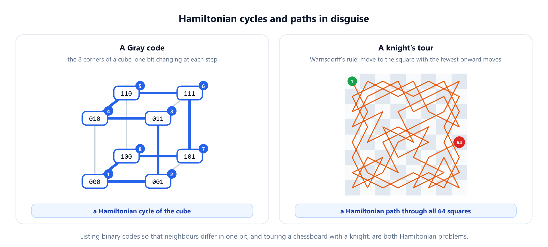
n, joined when they differ in one bit, is Hamiltonian forn ≥ 2. A Hamiltonian cycle of it is a Gray code: a list of all2nstrings in which consecutive strings differ in a single bit. Frank Gray patented the reflected binary code in 1953 for signal transmission. - Knight's tours. A knight that visits every square of a chessboard once traces a Hamiltonian path in the graph of knight moves. Euler studied such tours in 1759, Warnsdorff proposed in 1823 the rule of always moving to the square with the fewest onward moves, and Schwenk determined in 1991 exactly which rectangular boards have a closed tour.
10. Random graphs: when do Hamiltonian cycles appear?
The obstructions in section 3 are mostly local: a vertex with only one edge, or a few vertices that cut a piece of the graph off. In random graphs the local obstruction turns out to be the only one that matters. Pósa proved in 1976 that a random graph on n vertices with about C n log n edges, for a suitable constant C, is almost surely Hamiltonian. Komlós and Szemerédi found the exact threshold in 1983: it is where the expected number of vertices of degree less than 2 drops to zero.
The sharpest form is a statement about a graph growing one random edge at a time. Bollobás in 1984, and independently Ajtai, Komlós and Szemerédi in 1985, proved that with probability tending to 1, the graph becomes Hamiltonian at exactly the moment its last vertex of degree less than 2 disappears. In a random graph, once nothing obviously blocks a Hamiltonian cycle, one exists.
11. Where Hamiltonian paths are used
- Routing and touring. Every delivery round, inspection route or drilling sequence that must visit each site once is a Hamiltonian cycle problem with distances attached, which is the travelling salesperson problem.
- Genome assembly. Early assemblers modelled DNA reads as vertices joined by overlaps and looked for a Hamiltonian path through them. Idury and Waterman proposed in 1995 to recast assembly as an Eulerian path problem in a de Bruijn graph, and Pevzner, Tang and Waterman developed the approach in 2001, which is why modern assemblers solve Euler's easy problem instead of Hamilton's hard one.
- Encoders and Gray codes. Rotary and linear position encoders use Gray codes so that moving from one position to the next changes a single bit, which avoids large reading errors during transitions.
- Testing and sequencing. Visiting every state of a system once, or ordering jobs so that each follows a compatible predecessor, are Hamiltonian path problems on the graph of allowed transitions.
- Puzzles. The Icosian game, knight's tours and many path-drawing puzzles ask for Hamiltonian paths or cycles in disguise.
12. Common mistakes
| Mistake | Why it is wrong | Fix |
|---|---|---|
| Confusing Hamiltonian with Eulerian | Euler uses every edge once; Hamilton visits every vertex once | Check which objects must be covered: edges or vertices |
| "Every vertex has degree 3, so a cycle exists" | The Petersen graph is 3-regular and has no Hamiltonian cycle | Use degree conditions only in their exact form, such as Dirac's n / 2 |
| Treating Dirac or Ore as necessary | A plain cycle has every degree 2 and is Hamiltonian | Read them as sufficient conditions only |
| Concluding a cycle exists because no obstruction was found | The Petersen graph has no small obstruction set and no cycle | An obstruction proves "no"; only a found cycle proves "yes" |
| Assuming a path implies a cycle | The museum and the Petersen graph have paths but no cycles | Check that the path's two ends are adjacent |
| Expecting backtracking to scale | 20! orderings is about 2.4 × 10¹⁸ | Prune hard, or use the O(2n n2) dynamic program |
| Thinking planarity or 3-regularity makes it easy | The problem stays NP-complete for 3-connected cubic planar graphs | Look for 4-connectivity, where Tutte's theorem applies |
13. Glossary
| Term | Meaning |
|---|---|
| Hamiltonian path | A path that visits every vertex exactly once |
| Hamiltonian cycle | A cycle that visits every vertex exactly once |
| Hamiltonian graph | A graph that has a Hamiltonian cycle |
| Traceable graph | A graph that has a Hamiltonian path |
| Hypohamiltonian graph | A non-Hamiltonian graph in which deleting any vertex leaves a Hamiltonian graph |
| Cut vertex | A vertex whose removal disconnects the graph |
| Toughness | A measure comparing how many pieces a graph falls into with how many vertices are removed |
| Closure | The graph obtained by joining non-adjacent pairs with degree sum at least n until none remain |
| Tournament | A directed graph with exactly one arrow between every two vertices |
| Gray code | An ordering of binary strings in which neighbours differ in one bit |
| Knight's tour | A sequence of knight moves visiting every square of a board once |
| Held–Karp algorithm | Dynamic programming over subsets, O(2n n2) time |
14. Frequently asked questions
What is a Hamiltonian path?
A Hamiltonian path is a path in a graph that visits every vertex exactly once. A Hamiltonian cycle does the same and returns to its starting vertex. A graph that has a Hamiltonian cycle is called Hamiltonian. The name comes from William Rowan Hamilton, whose 1857 Icosian game asked for such a cycle on the corners of a dodecahedron.
What is the difference between Hamiltonian and Eulerian paths?
An Eulerian path uses every edge exactly once, while a Hamiltonian path visits every vertex exactly once. Whether an Eulerian path exists can be decided in linear time by counting vertices of odd degree. No such test is known for Hamiltonian paths: deciding whether one exists is NP-complete.
How do you prove a graph has no Hamiltonian cycle?
Find a set of k vertices whose removal leaves more than k connected pieces, because a cycle with k vertices removed breaks into at most k arcs. A cut vertex is the case k = 1. Other quick proofs use vertices of degree 1 or bipartite graphs with sides of different sizes. Failing to find such a proof does not show a cycle exists, as the Petersen graph demonstrates.
What is Dirac's theorem?
Dirac's theorem of 1952 says that every simple graph with n vertices, where n is at least 3, in which every vertex has degree at least n/2, has a Hamiltonian cycle. Ore's theorem weakens the condition to deg(u) + deg(v) at least n for every pair of non-adjacent vertices. Both are sufficient conditions, not necessary ones.
Is the Hamiltonian path problem NP-complete?
Yes. Deciding whether a graph has a Hamiltonian cycle or a Hamiltonian path is NP-complete, and the cycle problem was on Karp's 1972 list of 21 NP-complete problems. It stays NP-complete even for planar, 3-connected graphs in which every vertex has degree 3.
What is the fastest algorithm for Hamiltonian cycles?
The classic exact method is the dynamic program of Bellman and of Held and Karp, which runs in O(2 to the power n times n squared) time by recording paths through every subset of vertices. For undirected graphs, a randomized algorithm by Björklund from 2014 runs in O*(1.657 to the power n) time, ignoring polynomial factors. In practice, backtracking with strong pruning often works well on sparse graphs.
15. References
The definitions, theorems and attributions above come from these sources, listed in chronological order.
- Euler, L. (1759). "Solution d'une question curieuse qui ne paroît soumise à aucune analyse." Mémoires de l'Académie Royale des Sciences et Belles Lettres de Berlin 15, 310 to 337. Dated 1759, printed 1766. Knight's tours.
- Warnsdorff, H. C. von (1823). Des Rösselsprunges einfachste und allgemeinste Lösung. Schmalkalden: Varnhagen.
- Kirkman, T. P. (1856). "On the Representation of Polyedra." Philosophical Transactions of the Royal Society of London 146, 413 to 418.
- Tait, P. G. (1884). "Listing's Topologie." Philosophical Magazine, 5th series, 17, 30 to 46.
- Petersen, J. (1898). "Sur le théorème de Tait." L'Intermédiaire des Mathématiciens 5, 225 to 227.
- Whitney, H. (1931). "A Theorem on Graphs." Annals of Mathematics 32(2), 378 to 390.
- Rédei, L. (1934). "Ein kombinatorischer Satz." Acta Litterarum ac Scientiarum Szeged 7, 39 to 43.
- Tutte, W. T. (1946). "On Hamiltonian Circuits." Journal of the London Mathematical Society 21(2), 98 to 101.
- Dirac, G. A. (1952). "Some Theorems on Abstract Graphs." Proceedings of the London Mathematical Society s3-2, 69 to 81.
- Gray, F. (1953). "Pulse Code Communication." US Patent 2,632,058.
- Tutte, W. T. (1956). "A Theorem on Planar Graphs." Transactions of the American Mathematical Society 82, 99 to 116.
- Camion, P. (1959). "Chemins et circuits hamiltoniens des graphes complets." Comptes Rendus de l'Académie des Sciences 249, 2151 to 2152.
- Ore, O. (1960). "Note on Hamilton Circuits." The American Mathematical Monthly 67(1), 55.
- Bellman, R. (1962). "Dynamic Programming Treatment of the Travelling Salesman Problem." Journal of the ACM 9(1), 61 to 63.
- Held, M. and Karp, R. M. (1962). "A Dynamic Programming Approach to Sequencing Problems." Journal of the Society for Industrial and Applied Mathematics 10(1), 196 to 210.
- Chvátal, V. and Erdős, P. (1972). "A Note on Hamiltonian Circuits." Discrete Mathematics 2(2), 111 to 113.
- Karp, R. M. (1972). "Reducibility Among Combinatorial Problems." In Complexity of Computer Computations, edited by R. E. Miller and J. W. Thatcher, 85 to 103. New York: Plenum.
- Chvátal, V. (1973). "Tough Graphs and Hamiltonian Circuits." Discrete Mathematics 5(3), 215 to 228.
- Bondy, J. A. and Chvátal, V. (1976). "A Method in Graph Theory." Discrete Mathematics 15(2), 111 to 135.
- Garey, M. R., Johnson, D. S. and Tarjan, R. E. (1976). "The Planar Hamiltonian Circuit Problem is NP-Complete." SIAM Journal on Computing 5(4), 704 to 714.
- Pósa, L. (1976). "Hamiltonian Circuits in Random Graphs." Discrete Mathematics 14(4), 359 to 364.
- Itai, A., Papadimitriou, C. H. and Szwarcfiter, J. L. (1982). "Hamilton Paths in Grid Graphs." SIAM Journal on Computing 11(4), 676 to 686.
- Komlós, J. and Szemerédi, E. (1983). "Limit Distribution for the Existence of Hamiltonian Cycles in a Random Graph." Discrete Mathematics 43(1), 55 to 63.
- Bollobás, B. (1984). "The Evolution of Sparse Graphs." In Graph Theory and Combinatorics, edited by B. Bollobás, 35 to 57. London: Academic Press.
- Ajtai, M., Komlós, J. and Szemerédi, E. (1985). "First Occurrence of Hamilton Cycles in Random Graphs." Annals of Discrete Mathematics 27, 173 to 178.
- Holton, D. A. and McKay, B. D. (1988). "The Smallest Non-Hamiltonian 3-Connected Cubic Planar Graphs Have 38 Vertices." Journal of Combinatorial Theory, Series B 45(3), 305 to 319.
- Schwenk, A. J. (1991). "Which Rectangular Chessboards Have a Knight's Tour?" Mathematics Magazine 64(5), 325 to 332.
- Idury, R. M. and Waterman, M. S. (1995). "A New Algorithm for DNA Sequence Assembly." Journal of Computational Biology 2(2), 291 to 306.
- Pevzner, P. A., Tang, H. and Waterman, M. S. (2001). "An Eulerian Path Approach to DNA Fragment Assembly." Proceedings of the National Academy of Sciences 98(17), 9748 to 9753.
- Björklund, A. (2014). "Determinant Sums for Undirected Hamiltonicity." SIAM Journal on Computing 43(1), 280 to 299.
- Diestel, R. (2017). Graph Theory, 5th edition. Graduate Texts in Mathematics 173. Berlin: Springer.
Search for a tour yourself
Draw the museum in the visualizer and run the Hamiltonian path finder. Watch the search back up at dead ends, then add the door between G and I and ask for a cycle.
Open the visualizer