
Table of Contents
- 1. Walks, trails, paths and cycles
- 2. Girth, circumference and graphs without cycles
- 3. Detecting a cycle in an undirected graph
- 4. Union-find: cycles one edge at a time
- 5. Directed graphs: three colours
- 6. Kahn's algorithm: cycles as a stuck topological sort
- 7. How many cycles? The cycle space
- 8. Odd cycles and bipartite graphs
- 9. Eulerian circuits and Hamiltonian cycles
- 10. Cycles with weights: negative cycles
- 11. Cycles in a sequence: the tortoise and the hare
- 12. Where cycle detection matters
- 13. Common mistakes
- 14. Glossary
- 15. Frequently asked questions
- 16. References
1. Walks, trails, paths and cycles
A cycle is a route through a graph that comes back to where it started without reusing anything on the way. That sounds simple, but "route" can mean four different things, and most confusion about cycles comes from mixing them up. They differ only in what may repeat.
- A walk is a sequence of vertices in which each consecutive pair is joined by an edge. Vertices and edges may both repeat. Its length is the number of edges it uses, counted with repetition.
- A trail is a walk that never uses the same edge twice. Vertices may still repeat.
- A path is a walk that never visits the same vertex twice, so it cannot repeat an edge either.
- A walk is closed when it ends where it began. A closed trail is also called a circuit, and a cycle is a closed trail of positive length whose only repeated vertex is the one where it starts and ends.
Textbooks do not all use these words the same way. Some say "path" for what is called a walk here, and some say "circuit" for what is called a cycle. The ideas are stable even when the names are not, so when you read a theorem, check which one is meant. In a simple graph a cycle needs at least three vertices. In a multigraph a loop is a cycle of length 1 and two parallel edges form a cycle of length 2.
One undirected graph carries most of the article. It has eight vertices and ten edges: a triangle A, B, C on top, two squares B, C, E, D and D, E, G, F stacked below it, and a vertex H hanging off G.
V = {A, B, C, D, E, F, G, H}                          8 vertices
E = {AB, BC, CA, BD, CE, DE, DF, EG, FG, GH}          10 edges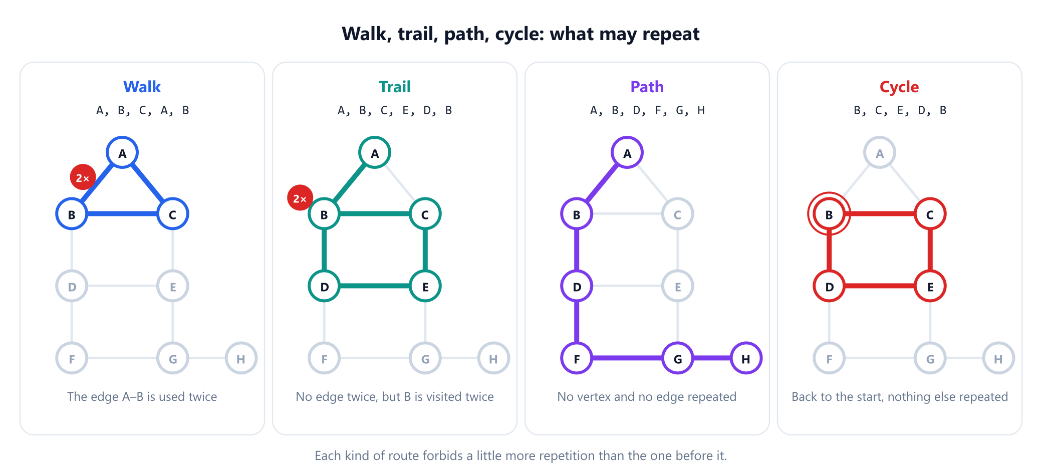
Two facts about closed walks are used again and again. First, a closed walk need not contain a cycle: A, B, A is closed, but it only goes out along one edge and back along the same edge. Second, a closed trail of positive length always contains a cycle. If it repeats some vertex in the middle, cut it there into two shorter closed trails and repeat the argument on either one; the process stops at a closed trail with no repeated vertex, which is a cycle. Section 8 needs a variant of the same argument for walks of odd length.
2. Girth, circumference and graphs without cycles
The girth of a graph is the length of its shortest cycle, and the circumference is the length of its longest. The example has six cycles in all, of lengths 3, 4, 4, 5, 6 and 7, so its girth is 3 and its circumference is 7. The longest cycle, A, B, D, F, G, E, C, passes through every vertex except H, which has only one edge and so can lie on no cycle at all.
| Graph | Girth | Why |
|---|---|---|
Complete graph Kn, n ≥ 3 | 3 | Any three vertices form a triangle |
Complete bipartite Km,n, m, n ≥ 2 | 4 | Every cycle alternates sides, so it is even |
| Petersen graph | 5 | Ten vertices of degree 3, and no triangle or square |
| A tree or forest | none | No cycle at all; the girth is often taken to be infinite |
A graph with no cycle is called acyclic. An acyclic undirected graph is a forest, and a connected forest is a tree. A forest on n vertices with k components has exactly n − k edges, so edge counting gives the quickest cycle test there is:
A graph withnvertices,medges andkcomponents contains a cycle if and only ifm > n − k. In particular, any graph with at least as many edges as vertices has a cycle.
The example has 10 > 8 − 1, so it must contain a cycle before anyone looks for one. A degree condition works too: if every vertex has degree at least 2, the graph has a cycle, and in fact one of length at least δ + 1, where δ is the minimum degree. The proof is a classic. Take a longest path v0, v1, …, vℓ. Every neighbour of v0 lies on the path, since otherwise the path could be made longer. v0 has at least δ neighbours on it, so the farthest one is at least vδ, and the edge back to it closes a cycle of length at least δ + 1, an observation that appears in Dirac's paper of 1952. This was checked by brute force on every graph with up to six vertices.
In a directed graph a cycle must follow the arrows, and an acyclic directed graph is called a DAG. DAGs are exactly the directed graphs whose vertices can be put in a line with every arrow pointing forwards, which is what a topological sort produces. Note that a DAG can have many edges: the edge-count test above is for undirected graphs only.
Finding the girth is harder than finding some cycle. Running a breadth-first search from every vertex and checking each non-tree edge it meets gives the girth in O(nm) time. Itai and Rodeh's 1978 paper on minimum circuits gives this bound, together with a faster method for a cycle at most one edge longer than the shortest.
3. Detecting a cycle in an undirected graph
If you only need a yes or no, the edge count settles it: compute the components and compare m with n − k. Usually you want more, namely an actual cycle you can show to someone. A cycle is a certificate: anyone can check it edge by edge, and it proves the answer without asking them to trust your program. Depth-first search produces one almost for free.
The key fact is that a depth-first search of an undirected graph sorts every edge into one of two kinds. A tree edge leads to a vertex seen for the first time. A back edge leads to a vertex already on the way down, an ancestor of the current one. There are no other kinds, so the graph has a cycle exactly when the search meets a back edge, and the cycle is the back edge plus the tree path it jumps over.
def find_cycle_undirected(vertices, edges):
    """Return the vertices of one cycle, in order, or None if the graph is a forest."""
    adj = {v: [] for v in vertices}
    for i, (u, v) in enumerate(edges):
        adj[u].append((v, i))
        adj[v].append((u, i))
    parent = {}                                   # vertex -> (parent vertex, edge id)
    for root in vertices:                         # one search per component
        if root in parent:
            continue
        parent[root] = (None, None)
        stack = [(root, iter(adj[root]))]
        while stack:
            u, it = stack[-1]
            for v, i in it:
                if i == parent[u][1]:             # the edge we arrived by, not a cycle
                    continue
                if v in parent:                   # back edge u-v: walk up from u to v
                    cycle = [u]
                    while cycle[-1] != v:
                        cycle.append(parent[cycle[-1]][0])
                    return cycle[::-1]
                parent[v] = (u, i)
                stack.append((v, iter(adj[v])))
                break
            else:
                stack.pop()
    return None

V = 'ABCDEFGH'
E = ['AB', 'BC', 'CA', 'BD', 'CE', 'DE', 'DF', 'EG', 'FG', 'GH']
print(find_cycle_undirected(V, E))
# ['A', 'B', 'C']
print(find_cycle_undirected(V, ['AB', 'BC', 'CE', 'DE', 'DF', 'FG', 'GH']))
# None
print(find_cycle_undirected('xy', ['xy', 'xy']))
# ['x', 'y']
Three details make this correct rather than nearly correct. The search remembers the edge it arrived by and skips only that edge; without the skip, every edge would look like a cycle of length 2, going out and straight back. Skipping by edge identity rather than by "the neighbour that is my parent" keeps the code right for multigraphs, where a doubled edge really is a cycle of length 2, as the third call shows. The outer loop starts one search per component, because a cycle can sit in any of them. And the stack is explicit, so a long path cannot overflow Python's recursion limit.
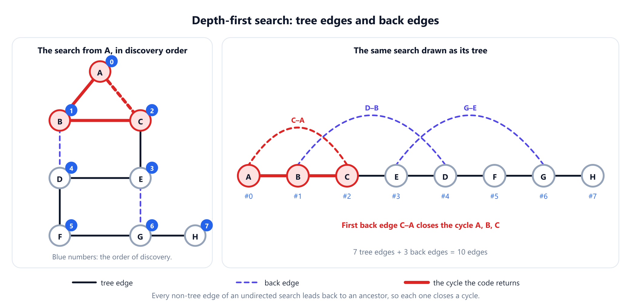
With neighbours taken in alphabetical order, the search from A walks down A, B, C and at C finds the edge back to A. A is already visited and the edge is not the one the search arrived by, so the code climbs the parent pointers from C to A and returns the triangle. Had it kept going, the search would have continued E, D, F, G, H, a single path through all eight vertices, and found two more back edges, D–B and G–E. Seven tree edges plus three back edges account for all ten.
There is a pleasant bonus in the running time. Before the first back edge, every adjacency entry the search reads is either a tree edge, at most n − 1 of them, or the edge back to a parent, at most n − 1 again. So the search itself reads at most 2n − 1 entries before it either finds a cycle or finishes, however many edges the graph has. That bound was checked by counting on 4,000 random graphs. Reading the input to build the adjacency lists still costs O(V + E), but the search does not.
4. Union-find: cycles one edge at a time
Sometimes the edges arrive one by one and the question is which edge first creates a cycle. A union-find structure answers that without any search. It keeps the vertices in groups, one group per component built so far. An edge between two different groups merges them. An edge whose two ends are already in the same group joins two vertices that were already connected, so together with the existing path between them it closes a cycle.
def first_cycle_edge(vertices, edges):
    """Add edges one at a time; return the first edge that closes a cycle, or None."""
    root = {v: v for v in vertices}
    def find(x):
        while root[x] != x:
            root[x] = root[root[x]]               # path halving
            x = root[x]
        return x
    for u, v in edges:
        ru, rv = find(u), find(v)
        if ru == rv:                              # u and v were already connected
            return u + v
        root[ru] = rv
    return None

print(first_cycle_edge('ABCDEFGH', ['AB', 'BD', 'DF', 'FG', 'GH', 'BC', 'CE', 'EG', 'DE', 'CA']))
# EG
In this order the first five edges form the path A, B, D, F, G, H, then B–C and C–E hang two more vertices on it. When E–G arrives, E and G already share a root, and the cycle it closes is B, C, E, G, F, D, six edges long. This is exactly the test Kruskal's algorithm applies to every edge before adding it to a minimum spanning tree.
Union-find tells you which edge closes a cycle, not where the cycle runs. To produce the cycle you still need the path between the two ends in the forest built so far, which a short search over the accepted edges finds. And union-find only works for undirected graphs. In the directed graph with arrows A→B, B→C and A→C, the third arrow joins two vertices that are already in one group, yet there is no directed cycle: following the arrows never leads back to A.
Watch a back edge close a cycle
Draw the triangle and the two squares, run the cycle detector, and see the search stop at the first edge that leads back to a vertex it has already visited.
Open the cycle detector5. Directed graphs: three colours
In a directed graph the undirected test gives wrong answers. Take six tasks with these dependencies:
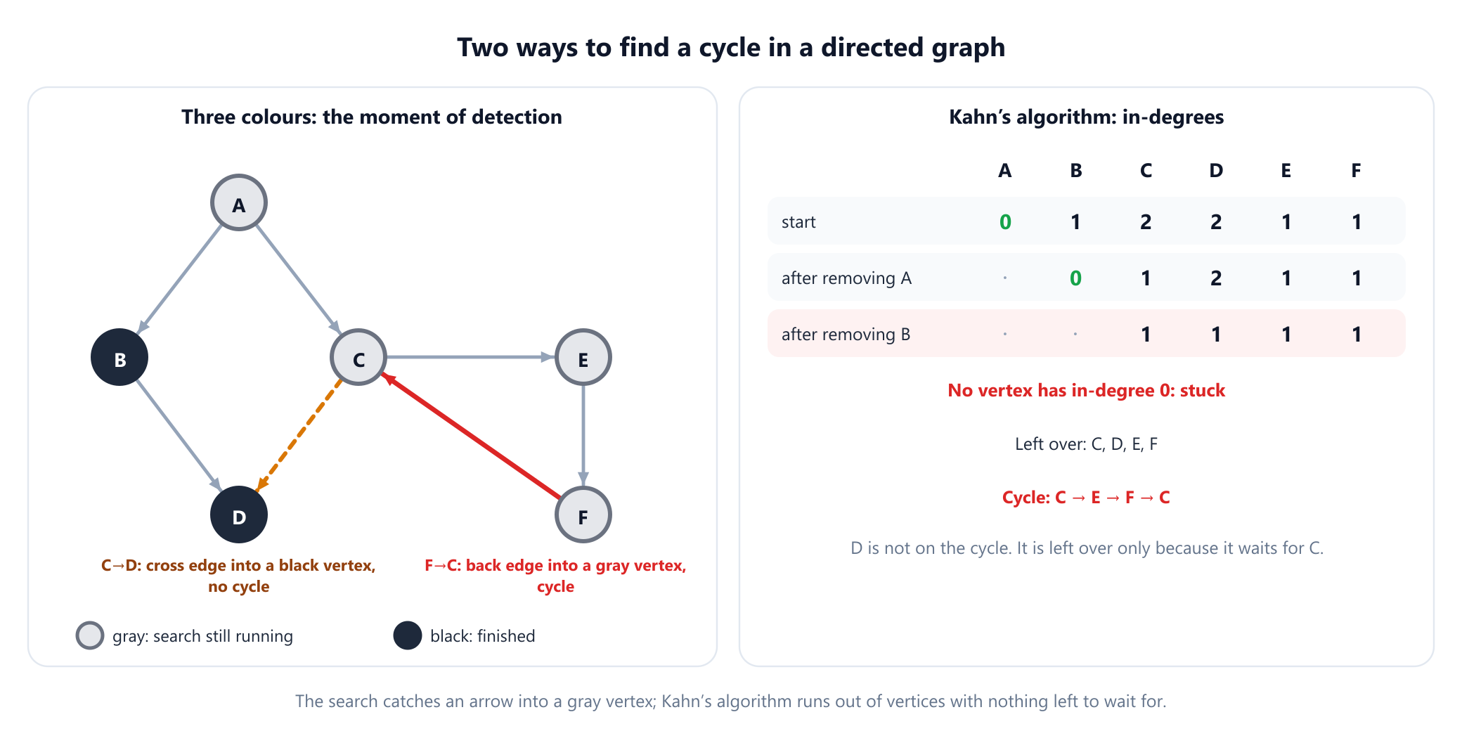
A → B A → C B → D C → D C → E E → FA depth-first search from A reaches D through B. Later, exploring C, it meets the arrow C→D and finds D already visited. A plain "already visited" check calls that a cycle, but there is none: A→B→D and A→C→D are two routes to the same place, not a route that comes back. On 6,000 random directed graphs, the plain check reported a cycle in 1,320 graphs that had none.
The fix is to remember not just whether a vertex was visited, but whether its search is still running. Each vertex gets one of three colours:
- WHITE: not reached yet.
- GRAY: reached, and its search has not finished. The gray vertices are exactly the current path from the root down to the vertex being explored.
- BLACK: finished. Everything reachable from it has been explored, and no cycle was found there.
A directed depth-first search sorts edges into four kinds: tree edges to white vertices, back edges to gray ancestors, forward edges to black descendants, and cross edges to black vertices in another branch or an earlier search. Only a back edge closes a cycle, because only a gray vertex is guaranteed to reach the current one. That gives the classic theorem: a directed graph has a cycle if and only if a depth-first search finds a back edge, which is the same as finding an arrow into a gray vertex. The gray path itself is the certificate.
WHITE, GRAY, BLACK = 0, 1, 2

def find_cycle_directed(graph):
    """Return one directed cycle as a list of vertices, or None if the graph is a DAG."""
    color = {v: WHITE for v in graph}
    for root in graph:
        if color[root] != WHITE:
            continue
        color[root] = GRAY
        path = [root]                             # the GRAY vertices, in order
        stack = [iter(graph[root])]
        while stack:
            for v in stack[-1]:
                if color[v] == GRAY:              # back edge: v is on the current path
                    return path[path.index(v):]
                if color[v] == WHITE:
                    color[v] = GRAY
                    path.append(v)
                    stack.append(iter(graph[v]))
                    break
            else:                                 # every out-edge done: finish the vertex
                color[path.pop()] = BLACK
                stack.pop()
    return None

dag = {'A': ['B', 'C'], 'B': ['D'], 'C': ['D', 'E'], 'D': [], 'E': ['F'], 'F': []}
print(find_cycle_directed(dag))
# None
dag['F'].append('C')                              # one more edge: F -> C
print(find_cycle_directed(dag))
# ['C', 'E', 'F']
On the six tasks, D turns black before C is explored, so C→D is a cross edge and is correctly ignored. Add one arrow, F→C, and the picture changes: the search goes C, E, F, all gray, and the new arrow points back into C, which is still gray. The gray path from C to F is returned as the cycle. A loop v→v is handled too: v is gray when its own arrow is read, and the cycle returned is just [v].
6. Kahn's algorithm: cycles as a stuck topological sort
The second standard method needs no recursion and no colours. A vertex with in-degree 0 depends on nothing, so it can safely go first. Kahn's algorithm, published in 1962, repeatedly removes such a vertex and lowers the in-degrees of its successors. If every vertex is removed, the removal order is a topological order and the graph is a DAG. If the process stops early, the graph has a cycle.
from collections import deque

def kahn(graph):
    """Topological order if the graph is a DAG, else (None, a cycle)."""
    indeg = {v: 0 for v in graph}
    for u in graph:
        for v in graph[u]:
            indeg[v] += 1
    ready = deque(v for v in graph if indeg[v] == 0)
    order = []
    while ready:
        u = ready.popleft()
        order.append(u)
        for v in graph[u]:
            indeg[v] -= 1
            if indeg[v] == 0:
                ready.append(v)
    if len(order) == len(graph):
        return order, None
    left = {v for v in graph if indeg[v] > 0}     # every one of them has a predecessor in left
    pred = {v: u for u in left for v in graph[u] if v in left}
    v, seen = next(iter(sorted(left))), []
    while v not in seen:                          # walk backwards until a vertex repeats
        seen.append(v)
        v = pred[v]
    return None, seen[seen.index(v):][::-1]

graph = {'A': ['B', 'C'], 'B': ['D'], 'C': ['D', 'E'], 'D': [], 'E': ['F'], 'F': ['C']}
print(kahn(graph))
# (None, ['E', 'F', 'C'])
graph['F'] = []
print(kahn(graph))
# (['A', 'B', 'C', 'D', 'E', 'F'], None)
Why does getting stuck prove a cycle? Every vertex left over still has at least one incoming arrow, and that arrow comes from a leftover vertex, because every removed vertex has already subtracted its arrows from the counts. So from any leftover vertex you can step backwards along an arrow to a leftover vertex, forever. With finitely many vertices, the backward walk must repeat a vertex, and the stretch between the two visits is a cycle. The code does exactly that walk and reports E, F, C, the same cycle as before read from a different starting point.
One detail is easy to get wrong. On the example, Kahn's algorithm removes A and B, then stalls with C, D, E and F still in place. D is not on any cycle; it is stuck only because it waits for C. The leftover vertices are the cycles plus everything downstream of them, so reporting the leftover set as "the cycle" is a bug. Without the arrow F→C the same code returns the order A, B, C, D, E, F, one of nine valid orders of that DAG.
Both methods run in O(V + E) time. The depth-first version hands you a cycle directly, while Kahn's version hands you a topological order whenever one exists, which is usually what a scheduler or build tool wanted in the first place.
7. How many cycles? The cycle space
Counting cycles one by one quickly gets out of hand. The complete graph K4 has 7 cycles, K5 has 37, K6 has 197, and K10 has 556,014. Listing them all is possible, and Johnson's algorithm of 1975 does it for directed graphs in O((n + e)(c + 1)) time for c cycles, but the output alone can be exponential in the size of the graph.
There is a much better count. Think of a cycle as a set of edges, and combine two edge sets by symmetric difference: keep the edges that are in exactly one of them. Under this operation, the subgraphs in which every vertex has even degree form a vector space over the two-element field, called the cycle space. Every cycle lies in it, and its dimension is
the cyclomatic number, or circuit rank: m − n + k.
A basis is easy to build. Take any spanning forest, which has n − k edges. Each of the remaining m − n + k edges closes exactly one cycle with the forest, its fundamental cycle, and these cycles are independent because each contains an edge that no other one does. The idea goes back to Kirchhoff, who used it in 1847 to count the independent loop equations of an electrical network; the name cyclomatic number came later. A depth-first search delivers the basis directly: change the cycle finder so that it records every back edge instead of stopping at the first.
def cycle_basis(vertices, edges):
    """One cycle per non-tree edge of a DFS forest: m - n + k cycles in all."""
    adj = {v: [] for v in vertices}
    for i, (u, v) in enumerate(edges):
        adj[u].append((v, i))
        adj[v].append((u, i))
    parent, used, basis = {}, set(), []
    for root in vertices:
        if root in parent:
            continue
        parent[root] = None
        stack = [(root, iter(adj[root]))]
        while stack:
            u, it = stack[-1]
            for v, i in it:
                if i in used:                     # tree edge or a back edge already counted
                    continue
                used.add(i)
                if v in parent:                   # back edge: record its cycle, keep going
                    cycle = [u]
                    while cycle[-1] != v:
                        cycle.append(parent[cycle[-1]])
                    basis.append(cycle[::-1])
                    continue
                parent[v] = u
                stack.append((v, iter(adj[v])))
                break
            else:
                stack.pop()
    return basis

V = 'ABCDEFGH'
E = ['AB', 'BC', 'CA', 'BD', 'CE', 'DE', 'DF', 'EG', 'FG', 'GH']
basis = cycle_basis(V, E)
print(len(basis), len(E) - len(V) + 1, basis)
# 3 3 [['A', 'B', 'C'], ['B', 'C', 'E', 'D'], ['E', 'D', 'F', 'G']]

def edges_of(cycle):
    return {''.join(sorted(p)) for p in zip(cycle, cycle[1:] + cycle[:1])}
total = edges_of(basis[0]) ^ edges_of(basis[1]) ^ edges_of(basis[2])
print(sorted(total))
# ['AB', 'AC', 'BD', 'CE', 'DF', 'EG', 'FG']
The example has 10 − 8 + 1 = 3 independent cycles, and the search tree from section 3 produces the three most natural ones: the triangle and the two squares. Their symmetric difference cancels the shared edges B–C and D–E and leaves the outer cycle of length 7.
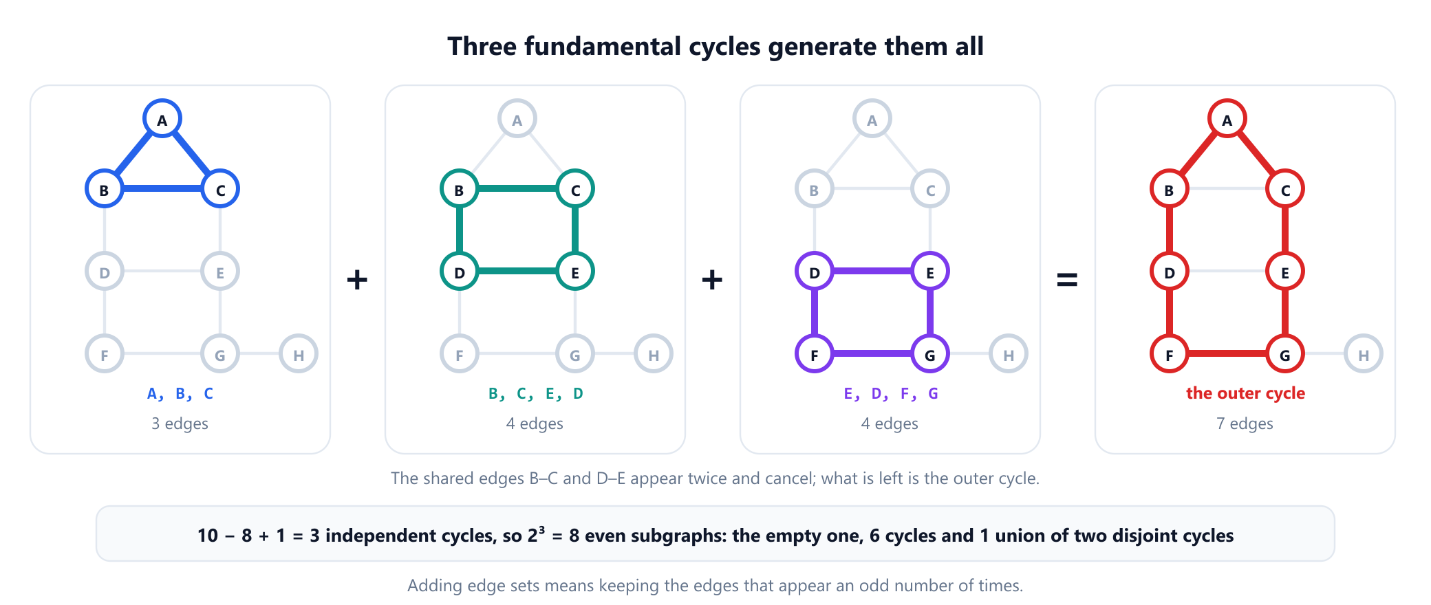
The space has 23 = 8 elements, and checking all of them is instructive. One is empty. Six are the six cycles of the graph. The last is the triangle together with the square D, E, G, F: every vertex has even degree, but the two cycles share no vertex, so the set is not a single cycle. Elements of the cycle space are edge-disjoint unions of cycles, not always cycles. For K10 the gap between the two counts is dramatic: a rank of 45 − 10 + 1 = 36, against 556,014 actual cycles.
The same number turns up in software engineering. McCabe's cyclomatic complexity of 1976 measures a program by the circuit rank of its control-flow graph, as E − N + 2P for E edges, N nodes and P connected pieces. The extra P comes from imagining one more edge from each exit back to its entry, which turns every path through the program into a cycle.
8. Odd cycles and bipartite graphs
The length of a cycle matters as much as its existence. A graph is bipartite, meaning its vertices split into two sides with every edge crossing between them, if and only if it has no odd cycle. One direction is immediate: a cycle alternates sides, so it returns home after an even number of steps. The other direction, proved by Kőnig in 1916, rests on this lemma:
Every closed walk of odd length contains a cycle of odd length.
Take a shortest odd closed walk. If it repeats a vertex in the middle, cut it there into two shorter closed walks. Their lengths add up to an odd number, so one of them is odd, contradicting the choice of the shortest. So the shortest odd closed walk repeats nothing, and it is an odd cycle. (Its length is at least 3, because a closed walk of length 1 would need a loop.)
In practice the test is a two-colouring by breadth-first search: colour the start vertex, give every neighbour the opposite colour, and look for an edge whose two ends get the same colour. When one is found, the two tree paths from its ends up to their nearest common ancestor, plus the edge itself, form an odd cycle, which is the certificate that no two-colouring exists. The example is not bipartite: three of its six cycles, of lengths 3, 5 and 7, are odd, and the triangle alone is enough to see it.
9. Eulerian circuits and Hamiltonian cycles
Two famous problems ask for special closed routes, and they sit on opposite sides of a deep divide.
- An Eulerian circuit uses every edge exactly once. It is a closed trail, not usually a cycle, since it may pass through a vertex many times. Euler's 1736 paper on the bridges of Königsberg showed that every vertex must then have even degree, and Hierholzer's paper of 1873 proved the converse: a connected graph, ignoring isolated vertices, has an Eulerian circuit exactly when all its degrees are even. The full story is in the guide to Eulerian paths and circuits.
- A Hamiltonian cycle visits every vertex exactly once. No comparable test is known. Deciding whether one exists is NP-complete, one of the 21 problems in Karp's 1972 list. Sufficient conditions exist, the best known being Dirac's theorem of 1952: a simple graph with
n ≥ 3vertices in which every vertex has degree at leastn/2has a Hamiltonian cycle.
The example fails both, for easy reasons. Six of its vertices, B, C, D, E, G and H, have odd degree, so it has no Eulerian circuit, and since more than two degrees are odd, not even an open Eulerian trail. And H has degree 1, so no cycle can pass through it; the best possible is the 7-cycle that misses only H. The Hamiltonian problem with distances attached is the travelling salesperson problem.
10. Cycles with weights: negative cycles
Once edges carry weights, a cycle has a total weight, and a negative cycle, one whose weights add up to less than zero, breaks shortest paths. Going around it once more always lowers the cost, so walks to any vertex reachable from the cycle have no shortest length at all. The Bellman-Ford algorithm detects this. A shortest path without a negative cycle has at most n − 1 edges, so after n − 1 rounds of relaxing every edge, all distances are final. If an n-th round still improves something, a negative cycle exists, and following the predecessor pointers back from an improved vertex leads into it.
A neat application is currency arbitrage. Give the edge from currency a to currency b the weight −log r, where r is the exchange rate. A round of trades multiplies money by the product of the rates, and the product exceeds 1 exactly when the sum of the weights is negative. A profitable loop is a negative cycle. When the question is the cycle with the smallest average weight per edge, Karp's 1978 characterisation of the minimum cycle mean solves it in O(nm) time.
11. Cycles in a sequence: the tortoise and the hare
A different kind of cycle detection works on graphs in which every vertex has exactly one outgoing edge. Following a linked list's next pointers, or applying a function f to a value again and again, walks such a graph. On a finite set the walk must eventually repeat a value, and from then on it repeats forever. The sequence looks like the Greek letter rho, ρ: a tail of length μ leading into a cycle of length λ.
Storing every value seen would find the repeat, but it costs memory proportional to μ + λ. The tortoise-and-hare method uses two pointers and nothing else. The tortoise moves one step at a time and the hare two. Once both are on the cycle, the hare gains one step per move, so it catches the tortoise within one lap. Knuth attributed the idea to Robert W. Floyd in 1969, although no paper by Floyd describing it is known.
def floyd(f, x0):
    """Tail length mu and cycle length lam of x0, f(x0), f(f(x0)), ... in O(1) memory."""
    tortoise, hare = f(x0), f(f(x0))
    while tortoise != hare:                       # 1. meet somewhere on the cycle
        tortoise, hare = f(tortoise), f(f(hare))
    mu, tortoise = 0, x0
    while tortoise != hare:                       # 2. walk in step to the cycle's entrance
        tortoise, hare = f(tortoise), f(hare)
        mu += 1
    lam, hare = 1, f(tortoise)
    while tortoise != hare:                       # 3. go once round the cycle
        hare = f(hare)
        lam += 1
    return mu, lam

f = lambda x: (x * x + 1) % 55
print(floyd(f, 0))
# (4, 6)
seq = [0]
for _ in range(11):
    seq.append(f(seq[-1]))
print(seq)
# [0, 1, 2, 5, 26, 17, 15, 6, 37, 50, 26, 17]
For f(x) = x2 + 1 mod 55 starting from 0, the values run 0, 1, 2, 5 and then enter the loop 26, 17, 15, 6, 37, 50, so μ = 4 and λ = 6. The two pointers first meet after six moves of the tortoise. The second phase works because at the meeting point the tortoise has taken some number t of steps and the hare 2t, so t is a multiple of λ. A pointer restarted at x0 and one left at the meeting point, both moving one step at a time, therefore arrive at the start of the cycle together after exactly μ steps.
The method takes O(μ + λ) time and constant memory. Brent's 1980 variant, which teleports the tortoise to the hare at powers of two, usually needs fewer evaluations of f. Both are used in Pollard's rho method for factoring integers, where f is a polynomial map such as x2 + c modulo the number being factored.
12. Where cycle detection matters
Whenever arrows mean "waits for", "depends on" or "refers to", a cycle means something cannot finish, cannot be built, or cannot be freed.
| Field | Vertices and arrows | A cycle means |
|---|---|---|
| Operating systems and databases | Processes or transactions, "waits for a resource held by" | A deadlock: nobody can proceed until someone gives up |
| Build systems and package managers | Modules or packages, "depends on" | No valid build order exists |
| Spreadsheets | Cells, "formula refers to" | A circular reference with no consistent value |
| Memory management | Objects, "holds a reference to" | Reference counts never reach zero, so plain reference counting leaks the cycle |
| Finance | Currencies, weighted by −log of the rate | A negative cycle is an arbitrage loop |
Deadlock is the textbook case. Coffman, Elphick and Shoshani listed four conditions in 1971 that must all hold for a deadlock to occur, and the last of them, circular wait, is in graph terms a cycle among the waiting tasks. A system can prevent deadlock by ruling out one of the conditions, for example by always acquiring locks in one fixed global order, which makes the wait-for graph a DAG. Or it can let deadlocks happen, look for a cycle from time to time, and break it by aborting one member.
Memory management is the same story in another form. A reference count drops to zero when the last pointer to an object goes away, but two objects that point at each other keep each other's counts at 1 even when nothing else can reach them. That is why CPython supplements reference counting with a separate collector whose job is to find such unreachable cycles.
13. Common mistakes
| Mistake | Why it is wrong | Fix |
|---|---|---|
| Treating the edge back to the parent as a cycle | Every undirected edge then looks like a cycle of length 2 | Skip the edge you arrived by |
| Skipping the parent vertex instead of the parent edge | A doubled edge in a multigraph, which is a real cycle, is missed | Skip the incoming edge by its identity |
| Using a visited set on a directed graph | Cross and forward edges to finished vertices raise false alarms | Use three colours and report only arrows into gray vertices |
| Using union-find on a directed graph | It ignores direction, so A→B, B→C, A→C looks cyclic | Use depth-first search or Kahn's algorithm |
| Reporting Kahn's leftover vertices as the cycle | They include everything downstream of a cycle, like D | Walk backwards inside the leftover set until a vertex repeats |
| Searching from one vertex only | A cycle in another component, or not reachable from the start, is never seen | Start a new search from every unvisited vertex |
| Recursing on a long path in Python | The default recursion limit of 1,000 is hit long before memory runs out | Use an explicit stack, as in the code above |
| Confusing a circuit with a cycle | An Eulerian circuit may pass through a vertex many times | Check which definition a theorem uses |
14. Glossary
| Term | Meaning |
|---|---|
| Walk | A sequence of vertices joined by edges; anything may repeat |
| Trail | A walk with no repeated edge |
| Path | A walk with no repeated vertex |
| Circuit | A closed trail |
| Cycle | A closed trail of positive length whose only repeated vertex is its start |
| Girth | The length of a shortest cycle |
| Circumference | The length of a longest cycle |
| Forest, tree | An acyclic graph; a connected acyclic graph |
| DAG | A directed acyclic graph |
| Back edge | An edge from a vertex to one of its ancestors in a depth-first search |
| Cycle space | The even-degree edge sets, combined by symmetric difference |
| Cyclomatic number, circuit rank | m − n + k, the dimension of the cycle space |
| Fundamental cycle | The cycle one non-tree edge closes with a spanning forest |
| Negative cycle | A cycle whose total weight is below zero |
15. Frequently asked questions
What is a cycle in a graph?
A cycle is a closed route that starts and ends at the same vertex, uses at least one edge, and repeats no other vertex and no edge. In a simple graph a cycle has at least three vertices; in a multigraph a loop is a cycle of length 1 and two parallel edges form a cycle of length 2. A graph with no cycle is acyclic: a forest if it is undirected, a DAG if it is directed.
How do you detect a cycle in an undirected graph?
Run a depth-first search that skips only the edge it arrived by. If the search reaches a vertex that is already visited, that edge is a back edge, and the back edge plus the tree path between its ends is a cycle. Alternatively, a graph with n vertices, m edges and k components has a cycle exactly when m > n − k, and union-find reports the first edge that closes one. All of these run in O(V + E) time.
How do you detect a cycle in a directed graph?
Use depth-first search with three colours: white for unvisited vertices, gray for vertices whose search is still running, and black for finished ones. An arrow into a gray vertex is a back edge and proves a cycle; arrows into black vertices do not. Kahn’s algorithm is the alternative: repeatedly remove vertices with in-degree 0, and if some vertices can never be removed, the graph has a cycle.
Why does a visited set give wrong answers on directed graphs?
In a directed graph a vertex can be reached twice along two different routes without any route coming back, as with A→B→D and A→C→D. A plain visited check calls the second arrival a cycle. Only an arrow into a vertex whose search is still in progress, a gray vertex, proves a cycle.
How many independent cycles does a graph have?
The cycle space of a graph with n vertices, m edges and k components has dimension m − n + k, called the cyclomatic number or circuit rank. For any spanning forest, each of the m − n + k edges outside it closes exactly one fundamental cycle, and every cycle is a symmetric difference of fundamental cycles. The total number of cycles can be far larger: K10 has rank 36 but 556,014 cycles.
Can union-find detect cycles in a directed graph?
No. Union-find ignores direction, so it treats the arrows A→B, B→C and A→C like a triangle and reports a cycle, although following the arrows never leads back to A. For directed graphs use depth-first search with three colours or Kahn’s algorithm.
16. References
The definitions, theorems and attributions above come from these sources, listed in chronological order.
- Euler, L. (1741). "Solutio problematis ad geometriam situs pertinentis." Commentarii academiae scientiarum Petropolitanae 8, 128 to 140. Volume dated 1736. The bridges of Königsberg and the degree condition for Eulerian circuits.
- Kirchhoff, G. (1847). "Ueber die Auflösung der Gleichungen, auf welche man bei der Untersuchung der linearen Vertheilung galvanischer Ströme geführt wird." Annalen der Physik und Chemie 72(12), 497 to 508. Spanning trees and one independent cycle per remaining edge.
- Hierholzer, C. (1873). "Ueber die Möglichkeit, einen Linienzug ohne Wiederholung und ohne Unterbrechung zu umfahren." Mathematische Annalen 6(1), 30 to 32. Published after the author's death.
- Kőnig, D. (1916). "Über Graphen und ihre Anwendung auf Determinantentheorie und Mengenlehre." Mathematische Annalen 77(4), 453 to 465. A graph is bipartite exactly when it has no odd cycle.
- Dirac, G. A. (1952). "Some Theorems on Abstract Graphs." Proceedings of the London Mathematical Society s3-2(1), 69 to 81.
- Bellman, R. (1958). "On a Routing Problem." Quarterly of Applied Mathematics 16(1), 87 to 90.
- Kahn, A. B. (1962). "Topological Sorting of Large Networks." Communications of the ACM 5(11), 558 to 562.
- Knuth, D. E. (1969). The Art of Computer Programming, Volume 2: Seminumerical Algorithms. Reading, MA: Addison-Wesley. Section 3.1, exercise 6, with the cycle-finding method attributed to Floyd.
- Coffman, E. G., Elphick, M. J. and Shoshani, A. (1971). "System Deadlocks." Computing Surveys 3(2), 67 to 78.
- Tarjan, R. E. (1972). "Depth-First Search and Linear Graph Algorithms." SIAM Journal on Computing 1(2), 146 to 160.
- Karp, R. M. (1972). "Reducibility Among Combinatorial Problems." In Complexity of Computer Computations, 85 to 103. New York: Plenum. Directed and undirected Hamiltonian circuit among the 21 NP-complete problems.
- Pollard, J. M. (1975). "A Monte Carlo Method for Factorization." BIT 15(3), 331 to 334.
- Johnson, D. B. (1975). "Finding All the Elementary Circuits of a Directed Graph." SIAM Journal on Computing 4(1), 77 to 84.
- McCabe, T. J. (1976). "A Complexity Measure." IEEE Transactions on Software Engineering SE-2(4), 308 to 320.
- Itai, A. and Rodeh, M. (1978). "Finding a Minimum Circuit in a Graph." SIAM Journal on Computing 7(4), 413 to 423.
- Karp, R. M. (1978). "A Characterization of the Minimum Cycle Mean in a Digraph." Discrete Mathematics 23(3), 309 to 311.
- Brent, R. P. (1980). "An Improved Monte Carlo Factorization Algorithm." BIT 20(2), 176 to 184. A faster cycle-finding method.
- Diestel, R. (2017). Graph Theory, 5th edition. Graduate Texts in Mathematics 173. Berlin: Springer.
Find a cycle yourself
Draw a graph, switch between directed and undirected, and watch the search report the first cycle it can prove. Then delete one edge of that cycle and run it again.
Open the visualizer