
Table of Contents
- 1. A weight is a function, not part of the graph
- 2. Unweighted means every weight is 1
- 3. The shortest path is not the shortest path
- 4. What a weight means: three ways they combine
- 5. Which algorithm the weights choose for you
- 6. Negative weights, and why Dijkstra breaks
- 7. Problems that only exist when weighted
- 8. Storing weights, and the zero-versus-infinity trap
- 9. Degree becomes strength
- 10. When to add weights, and when not to
- 11. Common mistakes
- 12. Glossary
- 13. Frequently asked questions
- 14. References
1. A weight is a function, not part of the graph
A graph is a pair of sets, G = (V, E), and nothing in that definition mentions numbers. Distances, costs, capacities and durations arrive from outside, as a separate function attached to the same edge set:
G = (V, E)                    the graph: which pairs are joined
w: E → ℝ                    the weight function: what each join costs
The standard texts are deliberate about this separation. Bondy and Murty define a weighted graph as a graph together with an assignment of a real number to each edge, and then define the weight of a subgraph as the sum of its edge weights, which is exactly what a shortest path or a minimum spanning tree minimises. Diestel treats weights the same way, as extra data laid over an unchanged combinatorial object.
Keeping w outside the graph is not pedantry, it buys three things:
- One graph can carry several cost models. A road network is one
Gwith three functions over it: kilometres, minutes, litres of fuel. Swapping the function changes every answer without touching a vertex or an edge. - Conditions attach to the function, not the structure. "Dijkstra needs non-negative weights" is a statement about
w. The graph is indifferent. - Structural results survive. Connectivity, planarity, bipartiteness, degree sequences and the handshaking lemma are properties of
(V, E)alone, so adding weights cannot change any of them.
An unweighted graph is then simply a graph with no such function supplied, and the next section shows that this is the same as supplying the most boring function there is.
2. Unweighted means every weight is 1
The cleanest way to hold the two cases in one head is to stop treating "unweighted" as the absence of weights and start treating it as a particular choice of them:
An unweighted graph is a weighted graph with w(e) = 1 for every edge. The weight of a path is then its number of edges, so "shortest path" means "fewest edges".
Everything follows from that single substitution. Breadth first search, which finds the fewest-edge path, is exactly what Dijkstra's algorithm degenerates into when every weight equals 1: the priority queue never needs to reorder anything, because distances come off it in non-decreasing integer order anyway, and a plain FIFO queue does the same job in O(n + m). Edward Moore's 1959 paper "The shortest path through a maze" posed and solved precisely this unit-weight problem, and is the paper the algorithm is usually traced back to.
The substitution runs the other way too, which is where the cost of weights shows up. Give the same graph arbitrary positive weights and the FIFO queue stops working, because a path with more edges can now be cheaper. You need a priority queue, and the running time goes from O(n + m) to O(m log n) with a binary heap, or O(m + n log n) with the Fibonacci heap of Fredman and Tarjan (1987).
3. The shortest path is not the shortest path
Here is the whole distinction in one picture. The same five vertices, the same five edges, asked the same question, give two different answers depending on whether the numbers are there.
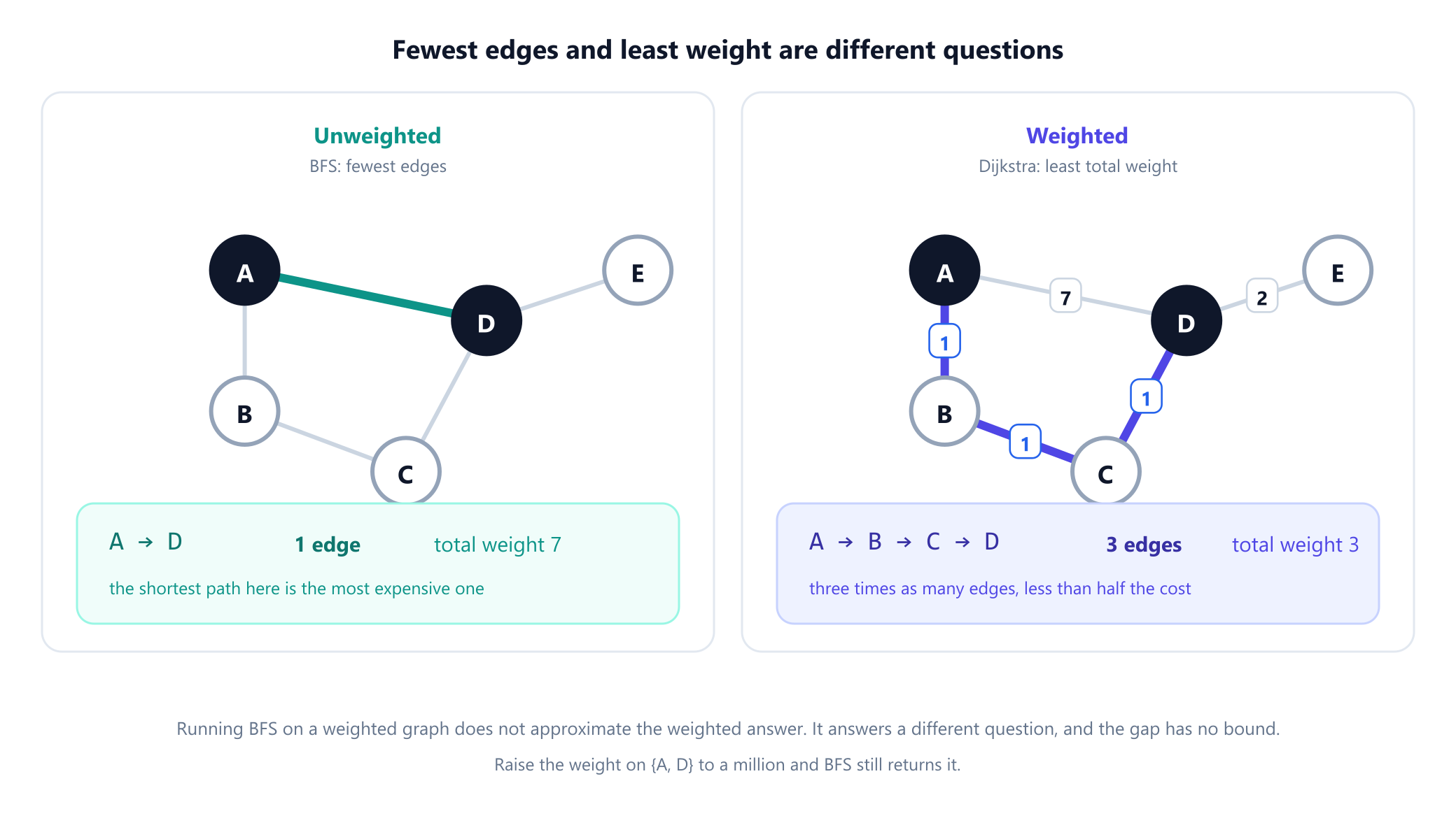
Written out, the graph is
V = {A, B, C, D, E}
E = { {A,B}, {B,C}, {C,D}, {A,D}, {D,E} }
w =    1       1       1       7       2
and the two questions have these answers:
| Question | Algorithm | Path found | Edges | Total weight |
|---|---|---|---|---|
| Fewest edges from A to D | BFS | A → D | 1 | 7 |
| Least total weight from A to D | Dijkstra | A → B → C → D | 3 | 3 |
| Fewest edges from A to E | BFS | A → D → E | 2 | 9 |
| Least total weight from A to E | Dijkstra | A → B → C → D → E | 4 | 5 |
Notice that the weighted answer uses more edges in both rows. That is the normal case, not a contrived one: a motorway detour is longer in junctions and shorter in minutes. Running BFS on a weighted graph does not give you an approximate answer, it gives you the answer to a different question, and the gap between them is unbounded. Raise the weight on {A, D} to a million and BFS still returns it.
4. What a weight means: three ways they combine
"Weighted graph" is a container, not a meaning. Before choosing an algorithm you have to answer a prior question: how do the weights along a path combine into the value you care about? There are three common answers and they lead to three different problems.
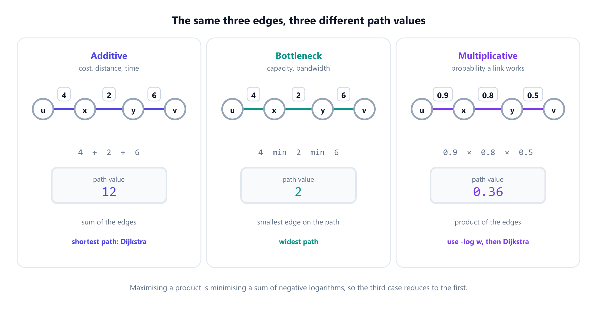
| Combination rule | Weight means | Path value | Problem and method |
|---|---|---|---|
| Additive | Distance, cost, time, hops | Sum of the edges | Shortest path: BFS, Dijkstra, Bellman-Ford |
| Bottleneck | Capacity, bandwidth, reliability of the weakest link | Minimum edge on the path | Widest path, also called maximin or minimax; solved by a modified Dijkstra or from a maximum spanning tree |
| Multiplicative | Probability a link works, transfer rates | Product of the edges | Most probable path: substitute -log w and it becomes additive |
The multiplicative trick is worth spelling out because it recurs everywhere from routing to natural language decoding. Maximising a product of probabilities along a path is the same as minimising the sum of their negative logarithms, since -log is monotone decreasing and turns products into sums. Because every probability is at most 1, every -log w is non-negative, so Dijkstra applies directly and no special algorithm is needed.
There is one more distinction that causes more modelling bugs than any of the above, and it is not about arithmetic at all:
Does a bigger number mean closer or further? In a distance graph, a large weight is bad and you minimise. In a similarity graph, a large weight is good and you maximise. The two are opposites, and the file format does not tell you which one you have.
Correlation networks, co-purchase graphs and embedding similarity graphs are all similarity-weighted, so feeding them to a shortest-path routine computes the path through the least similar links. If you need a distance from a similarity, convert deliberately: d = 1 - s for a similarity bounded in [0, 1], or d = 1/s, or d = -log s. Each choice changes the ranking of paths, so it is a modelling decision rather than a formality.
5. Which algorithm the weights choose for you
Once the combination rule is additive, the shape of the weight function alone decides the algorithm. This is the practical core of the weighted-versus-unweighted distinction.
| Weights | Use | Time | Why |
|---|---|---|---|
| All equal (unweighted) | BFS | O(n + m) | A FIFO queue already produces non-decreasing distances |
| Only 0 and 1 | 0-1 BFS with a deque | O(n + m) | Push a 0-edge to the front, a 1-edge to the back, and the deque stays sorted |
| Small integers, bounded by C | Dial's bucket queue | O(m + nC) | Buckets replace the heap when the range of distances is small |
| Arbitrary non-negative | Dijkstra | O(m log n), or O(m + n log n) with a Fibonacci heap | The greedy settle step needs distances to be non-decreasing |
| Any real, no negative cycle | Bellman-Ford | O(nm) | Relaxing every edge n-1 times needs no ordering assumption |
| Negative edges, all pairs | Johnson's algorithm | O(nm + n² log n) | Reweight once with Bellman-Ford so every weight becomes non-negative, then run Dijkstra from each vertex |
Two entries in that table deserve a note. 0-1 BFS is the neat observation that if weights are only 0 or 1 you never need a heap at all: a double-ended queue keeps the frontier sorted for free, which recovers linear time. Johnson's algorithm, from his 1977 paper in the Journal of the ACM, is the standard way to keep Dijkstra's speed on graphs with negative edges: it adds a potential function that makes every reweighted edge non-negative while preserving which paths are shortest.
There is also a striking result at the boundary of the unweighted case. Thorup showed in 1999 that single-source shortest paths on an undirected graph with positive integer weights can be solved in linear time, matching BFS, by exploiting the structure of integer weights rather than comparing distances. No comparable linear-time result is known for arbitrary real weights in the comparison-addition model, which is a reminder that "weighted" is not one problem but a family whose difficulty depends on what the weights look like.
6. Negative weights, and why Dijkstra breaks
Dijkstra's 1959 note assumed non-negative weights, and the assumption is load-bearing rather than decorative. The algorithm is greedy: once it removes a vertex from the queue it declares that vertex settled and never revisits it. That is sound only if no path discovered later can be cheaper, which is exactly what non-negativity guarantees, since extending a path can only add to its cost.
Introduce one negative edge and the guarantee fails. Here is a counterexample small enough to trace by hand, and free of ties so the pop order is forced:
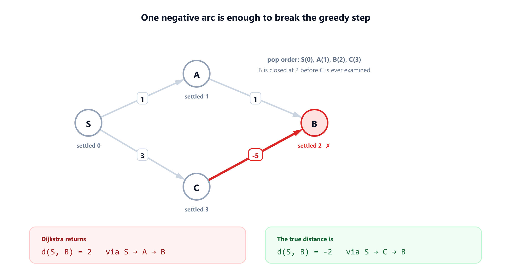
Trace it: the queue pops S at 0 and relaxes A to 1 and C to 3. It pops A at 1 and relaxes B to 2. It pops B at 2 and marks it settled. Only then does it pop C at 3 and find the arc C → B of weight -5, which would give B a distance of -2. Because B is already settled, the improvement is discarded and the algorithm reports 2 instead of -2.
Two clarifications that matter more than the counterexample itself:
- Negative weights are not the same as negative cycles. A graph can have negative edges and still have well-defined shortest paths, which is exactly the case Bellman-Ford handles in
O(nm). What breaks the problem entirely is a cycle of negative total weight, because you can go round it repeatedly and drive the cost to minus infinity. Bellman-Ford detects that condition rather than silently returning nonsense. - On an undirected graph a single negative edge is already a negative cycle. Walk along it and back and you have paid
2w < 0. So negative weights are effectively a directed-graph topic; on undirected graphs the shortest-walk problem becomes unbounded and the shortest-simple-path problem becomes NP-hard. The companion guide on directed versus undirected graphs covers that boundary.
Negative weights are not exotic. Arbitrage chains price currency conversions as products, which become sums of negative logarithms, and a profitable cycle appears in the model as a negative cycle. That is the standard textbook application of negative-weight detection, and it is why Bellman-Ford is worth its extra factor of n.
7. Problems that only exist when weighted
Some questions are not harder without weights, they are empty. The clearest case is the minimum spanning tree.
In an unweighted connected graph every spanning tree has exactly n - 1 edges, so every spanning tree is minimum and the problem is solved by any traversal: the BFS or DFS tree is already an answer. Add weights and the question becomes real, because spanning trees now have different total costs, and finding the cheapest is what Borůvka in 1926, Kruskal in 1956 and Prim in 1957 each solved.
On the running example the minimum spanning tree takes {A,B}, {B,C}, {C,D} and {D,E} for a total of 5, and rejects the expensive {A,D} at 7. Unweighted, all four spanning trees of that graph would be equally good.
| Problem | Unweighted | Weighted |
|---|---|---|
| Shortest path | Fewest edges, BFS in O(n + m) | Least total weight, Dijkstra or Bellman-Ford |
| Minimum spanning tree | Trivial: every spanning tree ties | The real problem: Kruskal, Prim, Borůvka |
| Maximum flow | Unit capacities, a special case | Capacities are the weights; the whole subject |
| Matching | Maximum cardinality matching | Maximum weight matching, a different algorithm |
| Widest path | Meaningless | Bottleneck objective, section 4 |
| Clustering and community detection | Based on edge presence | Based on edge strength, which changes the communities found |
| Centrality | Counts of paths and neighbours | Weighted variants; degree becomes strength, section 9 |
Maximum flow is the mirror image of the spanning tree case. Capacities are the weight function, so an unweighted flow network means unit capacities, which is the special case where max flow reduces to counting edge-disjoint paths by Menger's theorem. Ahuja, Magnanti and Orlin's Network Flows is the standard reference for the general weighted treatment, where each arc typically carries both a capacity and a cost, two weight functions on one graph.
8. Storing weights, and the zero-versus-infinity trap
Both standard representations extend in the obvious way, and both have a failure mode that is worth naming.
Adjacency matrix. Instead of 0 and 1, entry (u, v) holds the weight of that edge. The trap is immediate: what goes in the cells with no edge? Zero is the tempting default and it is wrong, because zero is a perfectly legal weight and the two cases become indistinguishable. Use ∞ for "no edge" in shortest-path contexts, since that is the identity for minimisation, and keep 0 on the diagonal. In an unweighted matrix the same cell means "no edge" with the value 0, which is precisely why code ported from unweighted to weighted breaks here.
unweighted        A[u][v] = 1 if joined, else 0
weighted          A[u][v] = w(u,v) if joined, else ∞      (0 on the diagonal)

sentinel bug      A[u][v] = 0 for "no edge" makes a zero-weight
                  edge invisible, and every distance collapse to 0
Adjacency list. Each entry becomes a pair rather than a bare vertex, so the list holds (neighbour, weight). Nothing else changes, and this is why the adjacency list is the default for weighted work: the memory overhead is one number per stored edge, and the traversal loop is identical.
A third format matters specifically for weighted graphs. The edge list of triples (u, v, w) is the natural input to Kruskal's algorithm, which sorts the whole list by weight, and to Bellman-Ford, which relaxes every edge in turn. Neither needs neighbour lookups, so neither needs an adjacency structure at all.
9. Degree becomes strength
Weights change descriptive statistics as well as algorithms. The weighted analogue of a vertex's degree is its strength, the sum of the weights of its incident edges:
deg(v)  =  number of incident edges          the unweighted count
s(v)    =  ∑ w(e)  over edges incident to v    the weighted total
Barrat, Barthélemy, Pastor-Satorras and Vespignani introduced the term in their 2004 PNAS paper on weighted networks, and the reason it matters is that the two quantities can rank vertices completely differently. An airport with many tiny regional routes has high degree and low strength; a hub with four enormous long-haul routes has low degree and high strength. Asking "which is the most important airport" gives a different answer depending on which you compute, and neither is wrong.
The same split runs through the rest of network analysis. Newman's 2004 paper "Analysis of weighted networks" shows how clustering coefficients, modularity and centrality all acquire weighted versions, and that the weighted and unweighted versions of a measure frequently disagree on the same data. When you report a network statistic, saying whether it used the weights is not a footnote, it is part of the definition.
10. When to add weights, and when not to
Weights are not free. They cost you linear-time algorithms, they add a modelling decision at every step, and they introduce scale sensitivity that an unweighted graph simply does not have. Reach for them when the answer genuinely depends on magnitude:
- Add weights when the edges are measurably unequal in a way that changes the decision: road lengths, link capacities, transaction amounts, correlation strengths, similarity scores.
- Stay unweighted when the relation is binary in nature (adjacency of countries, presence of a dependency), when the numbers you have are noisy proxies you would not defend, or when the question is purely structural, such as connectivity or bipartiteness.
- Threshold instead when weights exist but are unreliable. Keeping edges above a cutoff and discarding the rest turns a noisy weighted graph into a defensible unweighted one. State the cutoff, because results usually depend on it.
Two cautions specific to weighted data. First, scale matters: multiplying every weight by a positive constant leaves shortest paths and minimum spanning trees unchanged, since both minimise a sum, but it changes any statistic that compares weights against an absolute threshold, and a negative multiplier inverts the problem entirely. Second, units must agree before weights are added together. Mixing minutes with kilometres in one weight function produces numbers that no algorithm can interpret, and nothing in the code will complain.
11. Common mistakes
- Running BFS on a weighted graph. The most common of all. It returns the fewest-edge path, which is a correct answer to a different question, and the error is unbounded, as section 3 shows.
- Using 0 as the "no edge" sentinel. Fine until a genuine zero-weight edge exists, then silently wrong. Use infinity for minimisation problems.
- Feeding a similarity graph to a shortest-path routine. It will faithfully find the route through the weakest links. Convert similarity to distance first, and say how.
- Reaching for Dijkstra with negative weights. It does not merely lose optimality guarantees on some inputs, it returns concretely wrong numbers, as in section 6. Use Bellman-Ford, or Johnson for all pairs.
- Assuming a negative edge means a broken problem. Only a negative cycle makes shortest paths undefined. Bellman-Ford handles the rest and reports the cycle if one exists.
- Adding weights of different units. Minutes plus kilometres is meaningless, and no algorithm will tell you.
- Reporting a weighted network statistic without saying so. Degree and strength, and their derived centralities, routinely rank the same vertices differently.
- Forgetting that structure is unchanged. Connectivity, bipartiteness and degree sequences do not depend on
w. If a weighted algorithm gives an answer that contradicts one of them, the bug is in the weighting, not the theory.
12. Glossary
| Term | Meaning |
|---|---|
Weight function w: E → ℝ | Assigns a number to each edge; not part of G = (V, E) |
| Unweighted graph | Equivalently, a weighted graph with w(e) = 1 everywhere |
| Weight of a path | The sum of its edge weights, under the additive convention |
Distance d(u, v) | The minimum weight over all paths from u to v |
| Bottleneck value | The minimum edge weight along a path; maximised by the widest path |
| Negative cycle | A cycle of negative total weight; makes shortest paths undefined |
Strength s(v) | The sum of the weights of the edges at v, the weighted degree |
| Minimum spanning tree | A spanning tree of least total weight; trivial when unweighted |
| Reweighting | Shifting weights by a potential so they become non-negative, as in Johnson's algorithm |
| Thresholding | Turning a weighted graph unweighted by keeping only edges above a cutoff |
13. Frequently asked questions
What is the difference between a weighted and an unweighted graph?
A weighted graph carries a function w assigning a number to each edge, on top of the graph G = (V, E) itself. An unweighted graph has no such function, which is the same as every edge having weight 1. The practical consequence is that "shortest path" means fewest edges in the unweighted case and least total weight in the weighted case, and those are frequently different paths.
Can I use BFS on a weighted graph?
You can run it, and it will answer a different question: it returns the path with the fewest edges, ignoring the weights entirely. That is not an approximation of the least-weight path and the gap between them has no bound. Two exceptions are genuine: if every weight is equal, BFS is correct and faster than Dijkstra; and if the weights are only 0 and 1, a deque-based 0-1 BFS gives the correct weighted answer in linear time.
Why does Dijkstra's algorithm fail with negative weights?
Because it is greedy: when it removes a vertex from the priority queue it declares that distance final and never revisits it. That is sound only when extending a path cannot reduce its cost, which is exactly what non-negative weights guarantee. With a negative edge, a cheaper route can appear after the vertex has been settled, and the improvement is discarded. Section 6 gives a four-vertex example where Dijkstra returns 2 and the true distance is -2. Use Bellman-Ford instead, or Johnson's algorithm for all pairs.
Is a minimum spanning tree meaningful in an unweighted graph?
Not really. Every spanning tree of a connected graph on n vertices has exactly n-1 edges, so with equal weights they all have the same total and every spanning tree is minimum. Any BFS or DFS traversal already produces one in linear time. The minimum spanning tree problem only becomes interesting when the edges have different costs, which is why Kruskal's and Prim's algorithms are weighted algorithms by nature.
Do weights change whether a graph is connected?
No. Connectivity, bipartiteness, planarity, degree sequences and cycle structure are all properties of the pair (V, E) alone, and the weight function sits outside it. Adding, removing or rescaling weights cannot change any of them. If a weighted computation seems to contradict a structural fact, the error is in the weighting or the code, not in the theory.
How do I handle probabilities or similarities as weights?
Convert them to an additive cost first. For probabilities, the value of a path is the product of its edges, and maximising a product is the same as minimising the sum of negative logarithms, so replace w by -log w and run Dijkstra: every probability is at most 1, so every -log w is non-negative. For similarities, decide explicitly on a distance, such as 1 - s, 1/s or -log s. Feeding raw similarities to a shortest-path routine finds the path through the least similar links, which is almost never what was wanted.
14. References
The definitions, algorithms and attributions above come from these sources, listed in chronological order.
- Borůvka, O. (1926). "O jistém problému minimálním" (About a certain minimal problem). Práce Moravské Přírodovědecké Společnosti 3, 37 to 58. The earliest minimum spanning tree algorithm.
- Kruskal, J. B. (1956). "On the Shortest Spanning Subtree of a Graph and the Traveling Salesman Problem." Proceedings of the American Mathematical Society 7(1), 48 to 50.
- Prim, R. C. (1957). "Shortest Connection Networks and Some Generalizations." Bell System Technical Journal 36(6), 1389 to 1401.
- Bellman, R. (1958). "On a Routing Problem." Quarterly of Applied Mathematics 16(1), 87 to 90. Shortest paths that tolerate negative weights.
- Dijkstra, E. W. (1959). "A Note on Two Problems in Connexion with Graphs." Numerische Mathematik 1, 269 to 271. The non-negativity assumption is stated here.
- Moore, E. F. (1959). "The Shortest Path Through a Maze." Proceedings of an International Symposium on the Theory of Switching, Part II, 285 to 292. Harvard University Press. The unit-weight case, now known as BFS.
- Johnson, D. B. (1977). "Efficient Algorithms for Shortest Paths in Sparse Networks." Journal of the ACM 24(1), 1 to 13. Reweighting to remove negative edges.
- Fredman, M. L. and Tarjan, R. E. (1987). "Fibonacci Heaps and Their Uses in Improved Network Optimization Algorithms." Journal of the ACM 34(3), 596 to 615. Dijkstra in O(m + n log n).
- Ahuja, R. K., Magnanti, T. L. and Orlin, J. B. (1993). Network Flows: Theory, Algorithms, and Applications. Englewood Cliffs: Prentice Hall. The standard reference for capacities and costs as weights.
- Thorup, M. (1999). "Undirected Single-Source Shortest Paths with Positive Integer Weights in Linear Time." Journal of the ACM 46(3), 362 to 394.
- West, D. B. (2001). Introduction to Graph Theory, 2nd edition. Upper Saddle River: Prentice Hall.
- Barrat, A., Barthélemy, M., Pastor-Satorras, R. and Vespignani, A. (2004). "The Architecture of Complex Weighted Networks." Proceedings of the National Academy of Sciences 101(11), 3747 to 3752. Source of vertex strength.
- Newman, M. E. J. (2004). "Analysis of Weighted Networks." Physical Review E 70, 056131. Weighted versions of the standard network measures.
- Bondy, J. A. and Murty, U. S. R. (2008). Graph Theory. Graduate Texts in Mathematics 244. London: Springer. Source of the weighted-graph definition in section 1.
- Cormen, T. H., Leiserson, C. E., Rivest, R. L. and Stein, C. (2009). Introduction to Algorithms, 3rd edition. Cambridge, Massachusetts: MIT Press.
- Diestel, R. (2017). Graph Theory, 5th edition. Graduate Texts in Mathematics 173. Berlin: Springer.
Change one weight and watch the path move
Build the graph from section 3, run Dijkstra, then raise the weight on a single edge and run it again. Seeing the route jump is worth more than any amount of reading about it.
Open the visualizer