
Table of Contents
- 1. Two goals that pull in opposite directions
- 2. What a network costs: build and outages
- 3. The region used throughout
- 4. Step one: the cheapest tree
- 5. Junctions and the Steiner tree
- 6. Bridges: where one cut cuts customers off
- 7. Measuring reliability exactly
- 8. Surviving any single cut: the cheapest ring
- 9. Why patching the tree is not enough
- 10. Minimum cost against maximum reliability
- 11. The best design protects where it pays
- 12. What is a customer-hour worth?
- 13. What is easy, what is hard
- 14. What the model leaves out
- 15. From map to network plan
- 16. Mistakes that quietly cost money
- 17. Frequently asked questions
- 18. References
1. Two goals that pull in opposite directions
Every operator of a physical network, whether fibre, copper, power lines, water mains or gas pipes, faces the same planning question. Which links should be built so that every customer is connected, the construction bill is as small as possible, and a single digger, storm or failed joint does not leave thousands of people without service?
The two goals pull in opposite directions. The cheapest network that connects everyone has no spare routes at all, so every link is a single point of failure. The most reliable network builds every route that could be built, at a price no regulator or shareholder would accept. Good network design is finding where between the two a particular network should sit, and graph theory has precise tools for each part of the question.
The subject has deep roots in exactly these industries. Otakar Borůvka's 1926 algorithm for the cheapest connecting network was motivated by the electrification of Moravia, Robert Prim's 1957 paper on shortest connection networks came out of Bell Labs, and Edward Moore and Claude Shannon's 1956 study of reliable circuits built from unreliable relays started the mathematics of network reliability. Grötschel, Monma and Stoer's 1995 survey describes how survivable network design became a standard problem for telephone companies.
This article designs one regional network seven ways, from the cheapest tree to a proven optimum that balances construction against outages, and uses the same model to price reliability targets. Every number was computed by solving the model exactly, checking all 131,072 possible combinations of links, not estimated.
2. What a network costs: build and outages
Two numbers decide whether a network design is good:
- Build cost. Trenching, ducts and cable cost roughly the same per kilometre, adjusted for terrain. Here each kilometre costs $40,000. To compare a one-off build with yearly outages, the build is converted into an annual charge of 10% of its cost, standing for depreciation and the cost of capital.
- Outage cost. Buried cable gets cut, most often by construction work. Each link is cut on average 0.004 times per kilometre per year, one cut for every 250 km of cable each year, and each cut takes 12 hours to repair. A 50 km link is therefore out of service for 2.4 hours a year on average. When a town loses its connection to the exchange, every customer there loses service, and each customer-hour without service is valued at $5, standing for refunds, regulatory penalties, lost revenue and churn.
These figures are illustrative rather than taken from any operator, and section 12 shows how the answer changes when the value of a customer-hour is higher or lower. The structure, a one-off build cost against a recurring expected outage cost, is how survivable network design is usually framed.
3. The region used throughout
A regional exchange must connect seven towns. Cable can also meet at two roadside junction sites, J1 and J2, which serve no customers but can be used as meeting points.
| Town | Customers |
|---|---|
| Ashby | 4,200 |
| Brook | 3,100 |
| Colne | 5,600 |
| Dale | 2,400 |
| Everton | 6,100 |
| Fenwick | 1,800 |
| Garth | 3,300 |
That is 26,500 customers in total. Surveyors have identified 17 routes where cable could be laid, each with a length that follows roads and terrain rather than a straight line:
| Candidate link | Length, km | Build cost | Expected hours out of service per year |
|---|---|---|---|
| Exchange to J1 | 22.7 | $908k | 1.09 |
| Exchange to J2 | 31.3 | $1,252k | 1.50 |
| Exchange to Brook | 50.5 | $2,020k | 2.42 |
| Exchange to Everton | 60.5 | $2,420k | 2.90 |
| J1 to Ashby | 33.9 | $1,356k | 1.63 |
| J1 to Garth | 30.0 | $1,200k | 1.44 |
| J1 to Fenwick | 56.0 | $2,240k | 2.69 |
| J2 to Colne | 31.7 | $1,268k | 1.52 |
| J2 to Dale | 26.4 | $1,056k | 1.27 |
| J2 to Everton | 57.2 | $2,288k | 2.75 |
| Ashby to Brook | 45.5 | $1,820k | 2.18 |
| Brook to Colne | 53.6 | $2,144k | 2.57 |
| Colne to Dale | 62.4 | $2,496k | 3.00 |
| Dale to Everton | 50.8 | $2,032k | 2.44 |
| Everton to Fenwick | 50.6 | $2,024k | 2.43 |
| Fenwick to Garth | 48.4 | $1,936k | 2.32 |
| Garth to Ashby | 46.2 | $1,848k | 2.22 |
A design is any subset of these links. With 17 links there are 217 = 131,072 designs, of which 33,348 connect every town to the exchange. Building all 17 would cost $30.31 million.
4. Step one: the cheapest tree
Model the region as a weighted graph: sites are nodes, candidate links are edges, and each edge's weight is its build cost. The cheapest set of links that connects a set of nodes never contains a cycle, because removing any link from a cycle keeps everything connected and saves money. The answer is therefore a tree, and when it must reach every node it is a minimum spanning tree.
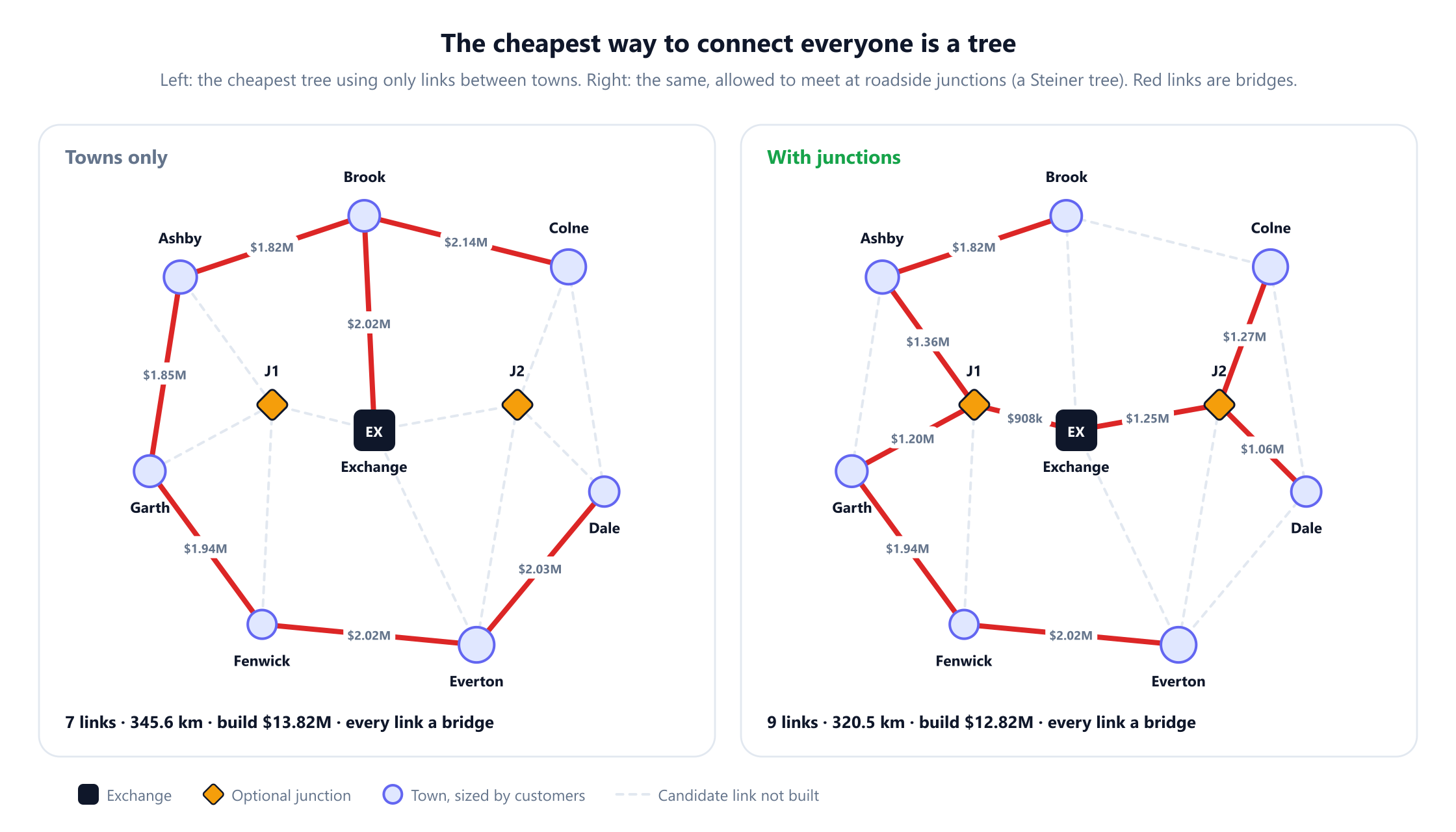
Kruskal's algorithm (1956) finds it by taking links from cheapest to most expensive and keeping each one that joins two parts not yet connected. Prim's algorithm (1957) grows the tree from one site, always adding the cheapest link to a new site. Both are fast and provably optimal. Using only links between the exchange and the towns, the cheapest tree has 7 links, 345.6 km, and costs $13.82 million.
5. Junctions and the Steiner tree
The junction sites do not need service, but cable is allowed to meet there, and that changes the problem. Connecting a required set of nodes, with the option of using extra nodes, is the Steiner tree problem, named after the geometric question of joining points with the shortest total road that Gilbert and Pollak surveyed in 1968.
With two junctions, the exact answer comes from trying each combination of junctions and finding the cheapest tree for each:
| Junctions allowed | Cheapest tree |
|---|---|
| None | $13,824k |
| J1 only | $13,420k |
| J2 only | $13,224k |
| Both | $12,820k |
Using both junctions, the cheapest tree has 9 links, 320.5 km, and costs $12.82 million, a saving of $1.004 million on the towns-only tree. Here running Kruskal over all ten sites happens to give the same tree, because both junctions are worth using. In general it does not: a spanning tree over every candidate site can include junctions that only add cost, and deciding which optional sites to use is what makes the Steiner tree problem hard. Richard Karp included it among his 21 NP-complete problems in 1972. The heuristic of Kou, Markowsky and Berman (1981), built on shortest paths and a minimum spanning tree, is guaranteed to be within a factor of two of the optimum, and Byrka and colleagues brought the best known guarantee down to about 1.39 in 2013.
6. Bridges: where one cut cuts customers off
A bridge is a link whose removal disconnects the network. In a tree every link is a bridge, which is the price of being cheapest. In the $12.82 million tree, a cut on the 22.7 km link between the exchange and J1 disconnects Ashby, Brook, Garth, Fenwick and Everton at once: 18,500 customers.
Robert Tarjan showed in 1974 how to find every bridge of a graph in a single depth-first search, in time proportional to the number of links. The same idea has a classical theorem behind it. Karl Menger proved in 1927 that the largest number of link-disjoint paths between two nodes equals the smallest number of links whose removal separates them, and Ford and Fulkerson's max-flow min-cut theorem (1956) turned this into an algorithm. In the tree, every town has exactly one path to the exchange. To survive any single cut, every town needs two paths that share no link.
7. Measuring reliability exactly
To price outages, each link is treated as out of service for its expected hours per year, independently of the others. The probability that a link is down at a random moment is those hours divided by the 8,760 hours in a year. A town is without service whenever the links that are working do not connect it to the exchange.
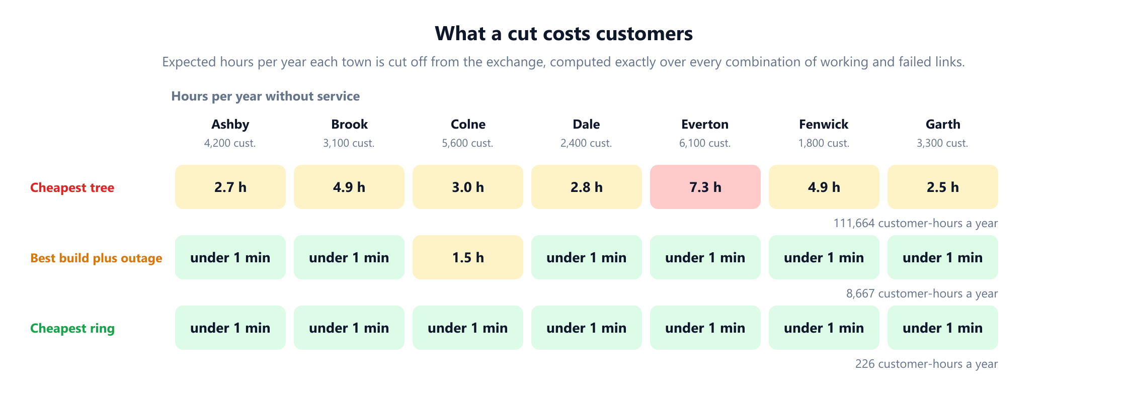
In a tree the calculation is intuitive: Everton's only route runs through J1, Garth and Fenwick, four links that are out of service for 7.3 hours a year between them, and Everton has the most customers of any town. Summed over all towns, the cheapest tree leaves customers without service for 111,664 customer-hours a year, about 4.2 hours for the average customer, which at $5 each is $558,319 a year.
For networks with loops the calculation is harder, because a town is cut off only by certain combinations of failures. The exact method used here checks every combination of working and failed links in a design, up to 217 of them, and adds up the probabilities of those that disconnect each town. That is feasible for one region but not for a national network: Leslie Valiant proved in 1979 that computing the probability that two nodes stay connected is #P-complete, and Provan and Ball (1983) proved the same for the whole network staying connected. Charles Colbourn's 1987 book surveys the bounds and approximations used in practice.
8. Surviving any single cut: the cheapest ring
A network that stays connected after any single link is cut is called 2-edge-connected, or survivable. It has no bridges, and by Menger's theorem every town has two link-disjoint paths to the exchange. Of the 33,348 connected designs, 2,460 are survivable, and checking all of them finds the cheapest.
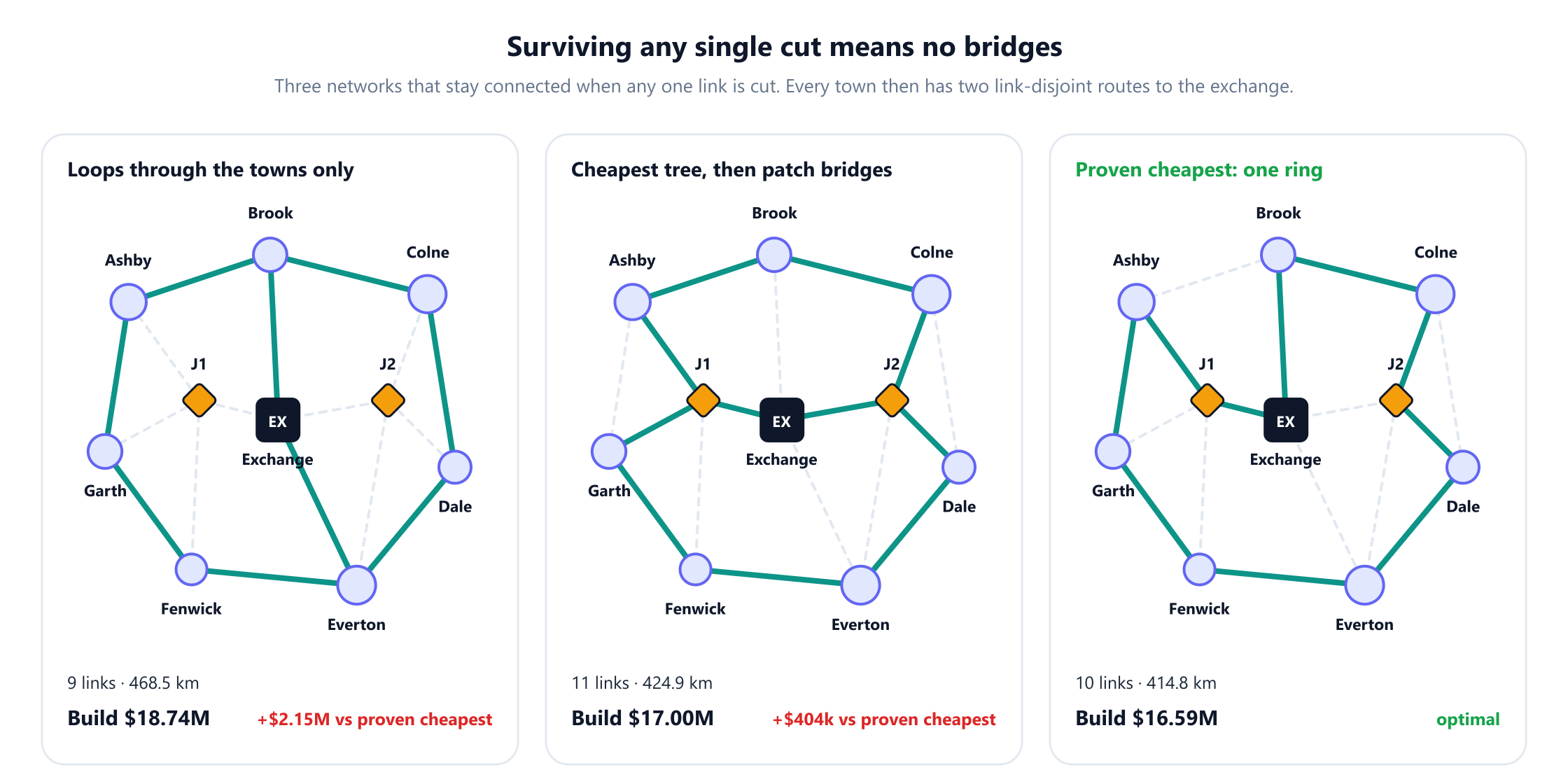
The cheapest survivable network costs $16.59 million and is a single ring: Exchange, J1, Ashby, Garth, Fenwick, Everton, Dale, J2, Colne, Brook and back to the exchange, 10 links and 414.8 km. It costs $3.77 million, or 29%, more than the cheapest tree, and it cuts expected outages from 111,664 to 226 customer-hours a year. In a ring, a town loses service only when both directions around the ring are cut at the same time.
That the optimum is a ring is not a coincidence. Rings are the standard survivable topology in telecommunications, from SONET and SDH self-healing rings to Ethernet ring protection, because traffic can be switched the other way round the ring within milliseconds of a cut. Monma, Munson and Pulleyblank (1990) studied minimum-cost survivable networks when link costs satisfy the triangle inequality, and showed that the cheapest tour through every site is then never far above the cheapest survivable network, which is part of the theoretical case for rings.
Without the junctions, the cheapest survivable design needs two loops through the towns and costs $18.74 million, $2.15 million more. The junctions that saved $1 million on the tree save more than twice as much on the survivable network.
9. Why patching the tree is not enough
A common way to add resilience is to start from the network that already exists, usually a tree, and add links until no bridge remains. A sensible greedy version adds, at each step, the link with the lowest cost per bridge removed.
From the $12.82 million tree, the greedy method first adds Dale to Everton for $2.03 million, which removes six bridges, then Brook to Colne for $2.14 million, which removes the last three. The result survives any single cut and costs $17.00 million, $404,000 more than the ring. The ring does not contain the tree: it drops three of the tree's links, Exchange to J2, J1 to Garth and Ashby to Brook, and uses Exchange to Brook and Garth to Ashby instead, together with the two links the greedy method added.
The patched network does have one advantage. With 11 links it has more redundancy than the ring, and its expected outage is 50 customer-hours a year against the ring's 226. Whether that is worth $404,000 depends on the value of a customer-hour, which is what the next sections measure.
Adding the fewest links to remove all bridges is solvable in polynomial time when every new link costs the same, as Eswaran and Tarjan showed in 1976. When links have different costs the problem is NP-hard, and Frederickson and JáJá (1981) gave approximation algorithms for it. The general lesson is the one this region illustrates: designing the tree first and reliability second locks in routes that a survivable design would not choose.
10. Minimum cost against maximum reliability
Survivability is a yes-or-no requirement, but reliability is a quantity. For every level of expected outage there is a cheapest design that achieves it, and plotting those designs gives the Pareto frontier: designs that cannot be made more reliable without costing more, or cheaper without being less reliable.
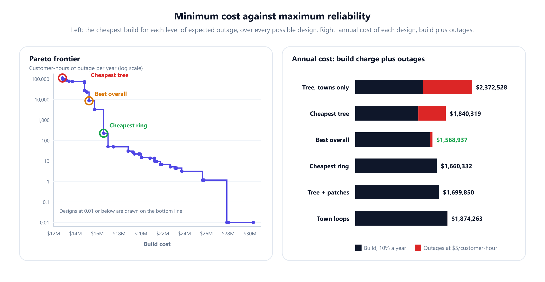
The frontier makes reliability targets concrete. The table reads off the cheapest design for several targets:
| Target: expected customer-hours of outage per year at most | Cheapest design | Its customer-hours | Build cost |
|---|---|---|---|
| No target | Cheapest tree | 111,664 | $12,820k |
| 2,000 | The ring | 226 | $16,592k |
| 500 | The ring | 226 | $16,592k |
| 100 | The patched tree | 50 | $16,996k |
| 20 | 12 links | 15 | $20,064k |
The steps get steeper. Going from the tree to the ring removes more than 111,000 customer-hours for $3.77 million. Going from the patched tree's 50 customer-hours to 15 costs another $3.07 million. In availability terms, the cheapest tree gives the average customer 99.95%, and the ring gives 99.9999%. Each additional "nine" of availability costs more than the last, which is why a reliability target should be chosen by pricing it, not by habit.
11. The best design protects where it pays
Adding each design's yearly build charge to its yearly outage cost at $5 per customer-hour, and checking all 33,348 connected designs, gives a single best design. It is neither the tree nor the ring.
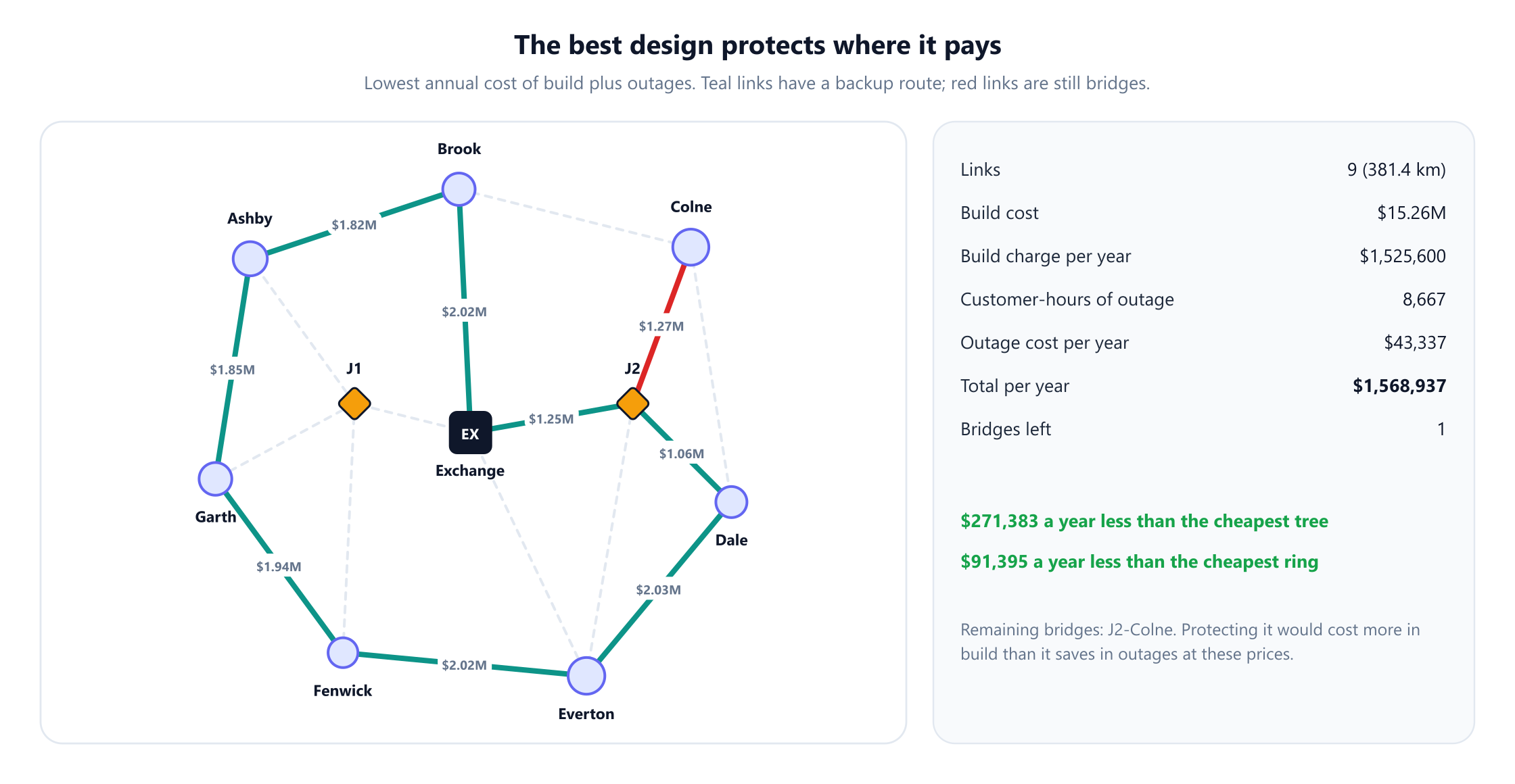
The best design costs $15.26 million to build: a loop through six towns and junction J2, with Colne connected by a single 31.7 km spur from J2. It leaves customers without service for 8,667 customer-hours a year, and its total yearly cost of $1,568,937 is $271,383 less than the cheapest tree and $91,395 less than the ring.
The surprise is which town is left unprotected. Colne has 5,600 customers, the second largest town. But its spur is short, out of service for about 1.5 hours a year, so its outages cost about $42,700 a year. Turning this design into the ring costs $1.336 million more to build, $133,600 a year, to remove 8,441 customer-hours worth $42,205. Protection pays where links are long, cuts are likely and many customers depend on one route. It does not pay simply because a town is large.
| Design | Build cost | Customer-hours per year | Total per year |
|---|---|---|---|
| Tree, towns only | $13,824k | 198,026 | $2,372,528 |
| Cheapest tree | $12,820k | 111,664 | $1,840,319 |
| Best overall | $15,256k | 8,667 | $1,568,937 |
| Cheapest ring | $16,592k | 226 | $1,660,332 |
| Tree plus patches | $16,996k | 50 | $1,699,850 |
| Loops through towns only | $18,740k | 53 | $1,874,263 |
The towns-only tree is the most expensive design in the table once outages are counted. It costs $1 million more to build than the cheapest tree and, because it strings Dale, Everton and Fenwick along long chains, it has 198,026 customer-hours of outage a year, almost twice as many.
12. What is a customer-hour worth?
The $5 figure is a judgement, and in practice it differs between a rural broadband network, a business fibre network with contractual service levels and an electricity grid where outages affect hospitals. Because the model checks every design, the best design can be found for every value at once. Each design's yearly cost is a straight line in the value of a customer-hour, and the best design is the lowest line:
| Value of a customer-hour | Best design | Build cost | Customer-hours per year | Bridges |
|---|---|---|---|---|
| Up to $2.61 | A tree | $12,828k | 99,022 | 9 |
| $2.61 to $2.69 | A tree | $13,028k | 91,347 | 9 |
| $2.69 to $9.38 | Loop, Colne on a spur | $15,256k | 8,667 | 1 |
| $9.38 to $27.63 | Loop, Dale on a spur | $15,768k | 3,209 | 1 |
| $27.63 to $228.96 | The ring | $16,592k | 226 | 0 |
| Above $228.96 | The patched tree, then larger networks | $16,996k and up | 50 and fewer | 0 |
Three things stand out. Even when outages are nearly free, the best tree is not the cheapest tree: for $8,000 more, a tree that reaches Everton through Dale instead of through Fenwick removes 12,642 customer-hours a year, so at any value above about 6 cents the $12.828 million tree wins. Second, full survivability is optimal only when a customer-hour is worth more than $27.63; between $2.69 and $27.63 the answer is a loop with one short spur. Third, the greedy patched tree, which was a poor survivable design, is the best design once a customer-hour is worth more than $228.96, because its extra link sharply reduces the double-cut outages the ring still has.
A planner who knows only that a customer-hour is worth "somewhere between $5 and $20" therefore learns that the decision is between two loops with one spur each, and that building the full ring would need a much higher outage value to justify it. That is more useful than any single optimum.
13. What is easy, what is hard
| Problem | Method | Difficulty |
|---|---|---|
| Cheapest tree reaching every site | Kruskal, Prim, Borůvka | Polynomial |
| Find all bridges | Depth-first search (Tarjan, 1974) | Linear time |
| Number of link-disjoint paths between two sites | Maximum flow (Menger, Ford and Fulkerson) | Polynomial |
| Minimum cuts between all pairs of sites | Gomory–Hu tree (1961) | Polynomial |
| Cheapest tree with optional junction sites | Steiner tree | NP-hard (Karp, 1972) |
| Cheapest survivable network | Contains the Hamiltonian cycle problem | NP-hard |
| Cheapest links to remove all bridges, different costs | Augmentation (Frederickson and JáJá, 1981) | NP-hard |
| Probability that sites stay connected | Network reliability | #P-complete (Valiant, 1979; Provan and Ball, 1983) |
Real networks have hundreds or thousands of sites, far too many to check every design. The survivable network design problem is solved with integer programming using cut constraints, as surveyed by Kerivin and Mahjoub (2005), with primal-dual approximation algorithms such as Jain's 2001 factor-two method for general connectivity requirements, and with heuristics tuned to telecommunications, described in Kershenbaum's 1993 textbook and Resende and Pardalos's 2006 handbook. The exhaustive search in this article plays the role of a benchmark: it shows exactly how far each simpler method is from the best possible.
14. What the model leaves out
- Shared trenches. Two cables in the same duct are cut by the same digger. Planners call these shared risk link groups, and two routes that share a trench are not really disjoint.
- Node failures. Junctions, cabinets and the exchange itself can fail. Protecting against those requires 2-vertex-connected designs, where every site has two paths that share no node.
- Capacity. After a cut, traffic moves to the surviving route, which must have room for it. Capacity planning turns the design into a multi-commodity flow problem.
- Correlated failures. Floods, storms and earthquakes cut many links at once, so the independence assumption understates the risk of rare large outages.
- Existing assets. Most projects extend a network that already exists, with ducts and poles that are much cheaper to reuse than new trenches.
- Regulation. Electricity grids are often planned to an N-1 criterion, which requires the system to keep supplying customers after the loss of any single element, the same idea as survivability applied to lines, transformers and generators.
None of these changes the core picture: sites as nodes, routes as weighted edges, bridges as single points of failure, and the choice between cost and reliability made by pricing both.
15. From map to network plan
Start with the candidate routes. The quality of a network design depends on the list of routes it is allowed to use. Include roadside cabinets, existing ducts, poles and rights of way as optional nodes and edges; in this region the two junctions saved $1 million on the tree and $2.15 million on the survivable design.
Price outages from real data. Fault records give cut rates per kilometre by area and cable type, and repair logs give repair times. Service level agreements, regulatory penalties and customer churn give the value of a customer-hour. When that value is uncertain, compute the best design across a range of values, as in section 12, rather than for one guess.
Design reliability in, do not bolt it on. Solving for cost and reliability together found a design $91,395 a year cheaper than the ring and $271,383 a year cheaper than the tree. Patching an existing tree cost $404,000 more than the best survivable design.
Use the right tools. Graph libraries such as NetworkX compute spanning trees, bridges and disjoint paths in a few lines. Mixed integer programming solvers such as HiGHS and Gurobi solve survivable design models with cut constraints for realistic regions, and specialised planning tools add geographic data and costing. Whatever the tool, check the bridges of every proposed plan: a single overlooked bridge is a single point of failure.
16. Mistakes that quietly cost money
- Connecting towns only to each other. Ignoring the junction sites made the tree $1 million dearer and the survivable network $2.15 million dearer.
- Treating the cheapest tree as the cheapest network. Once outages were counted, the cheapest tree cost $271,383 a year more than the best design.
- Choosing between two trees on build cost alone. Two trees $8,000 apart differed by 12,642 customer-hours a year.
- Patching bridges one at a time. The greedy patched tree cost $404,000 more to build than the ring.
- Requiring full survivability by default. At $5 per customer-hour the ring cost $91,395 a year more than a loop with one short spur.
- Protecting the biggest towns first. The best design left Colne, the second largest town, on a spur, because its route is short.
- Counting two cables in one trench as two routes. They fail together, so the network still has a bridge.
17. Frequently asked questions
What is network design optimization?
+
It is choosing which links of a physical network, such as fibre routes, power lines or pipes, to build so that every customer is connected at the lowest total cost, usually subject to reliability requirements. In graph terms, sites are nodes, candidate routes are weighted edges, and the task is to choose a subgraph that meets connectivity requirements at minimum cost, or that minimises the combined cost of construction and expected outages.
Why is a minimum spanning tree not enough for a telecom network?
+
A minimum spanning tree is the cheapest way to connect every site, but in a tree every link is a bridge, so a single cable cut disconnects every customer beyond it. In this article's example the cheapest tree left customers without service for 111,664 customer-hours a year. Once outages were priced, a design with one loop cost $271,383 a year less than the tree.
What is a bridge in a network?
+
A bridge is a link whose removal disconnects the network, so it is a single point of failure. Every link of a tree is a bridge. All bridges of a graph can be found in linear time with a depth-first search, as Tarjan showed in 1974. A network with no bridges is called 2-edge-connected and survives the loss of any single link.
Why are telecom networks built as rings?
+
A ring is the simplest network in which every site has two link-disjoint paths to every other, so traffic can be switched the other way round the ring when a cable is cut. It uses exactly as many links as sites, and when link costs satisfy the triangle inequality the cheapest ring is never far above the cheapest survivable network. In this article's example the cheapest survivable network was a single ring costing $16.59 million.
What is the Steiner tree problem?
+
It asks for the cheapest tree that connects a required set of nodes when other nodes, such as junctions or cabinets, may be used but do not have to be. Unlike the minimum spanning tree it is NP-hard, and good approximation algorithms exist. In the example, allowing cable to meet at two junctions reduced the cheapest tree from $13.82 million to $12.82 million.
How is network reliability calculated?
+
Each link is given a probability of being out of service, from its cut rate and repair time, and the reliability of a site is the probability that the working links still connect it to the source. For small networks it can be computed exactly by summing over every combination of working and failed links. In general the problem is #P-complete, so large networks use bounds, simulation or decomposition methods.
Should every network be designed to survive any single failure?
+
Not necessarily. Full survivability is the right target when outages are expensive, as in business networks or electricity grids planned to the N-1 criterion. In the example, a fully survivable ring was the cheapest choice overall only when a customer-hour of outage was worth more than $27.63. At $5, a loop that left one town on a short spur cost $91,395 a year less than the ring.
18. References
The foundational papers, surveys and books behind the methods in this article, in chronological order.
- Borůvka, O. (1926). “O jistém problému minimálním.” Práce moravské přírodovědecké společnosti, 3, 37–58.
- Menger, K. (1927). “Zur allgemeinen Kurventheorie.” Fundamenta Mathematicae, 10, 96–115.
- Ford, L. R. and Fulkerson, D. R. (1956). “Maximal flow through a network.” Canadian Journal of Mathematics, 8, 399–404.
- Kruskal, J. B. (1956). “On the shortest spanning subtree of a graph and the traveling salesman problem.” Proceedings of the American Mathematical Society, 7(1), 48–50.
- Moore, E. F. and Shannon, C. E. (1956). “Reliable circuits using less reliable relays.” Journal of the Franklin Institute, 262(3), 191–208.
- Prim, R. C. (1957). “Shortest connection networks and some generalizations.” Bell System Technical Journal, 36(6), 1389–1401.
- Gomory, R. E. and Hu, T. C. (1961). “Multi-terminal network flows.” Journal of the Society for Industrial and Applied Mathematics, 9(4), 551–570.
- Gilbert, E. N. and Pollak, H. O. (1968). “Steiner minimal trees.” SIAM Journal on Applied Mathematics, 16(1), 1–29.
- Karp, R. M. (1972). “Reducibility among combinatorial problems.” In R. E. Miller and J. W. Thatcher (eds.), Complexity of Computer Computations, 85–103. New York: Plenum.
- Tarjan, R. E. (1974). “A note on finding the bridges of a graph.” Information Processing Letters, 2(6), 160–161.
- Eswaran, K. P. and Tarjan, R. E. (1976). “Augmentation problems.” SIAM Journal on Computing, 5(4), 653–665.
- Valiant, L. G. (1979). “The complexity of enumeration and reliability problems.” SIAM Journal on Computing, 8(3), 410–421.
- Frederickson, G. N. and JáJá, J. (1981). “Approximation algorithms for several graph augmentation problems.” SIAM Journal on Computing, 10(2), 270–283.
- Kou, L., Markowsky, G. and Berman, L. (1981). “A fast algorithm for Steiner trees.” Acta Informatica, 15(2), 141–145.
- Provan, J. S. and Ball, M. O. (1983). “The complexity of counting cuts and of computing the probability that a graph is connected.” SIAM Journal on Computing, 12(4), 777–788.
- Colbourn, C. J. (1987). The Combinatorics of Network Reliability. New York: Oxford University Press.
- Monma, C. L., Munson, B. S. and Pulleyblank, W. R. (1990). “Minimum-weight two-connected spanning networks.” Mathematical Programming, 46, 153–171.
- Hwang, F. K., Richards, D. S. and Winter, P. (1992). The Steiner Tree Problem. Annals of Discrete Mathematics 53. Amsterdam: North-Holland.
- Kershenbaum, A. (1993). Telecommunications Network Design Algorithms. New York: McGraw-Hill.
- Grötschel, M., Monma, C. L. and Stoer, M. (1995). “Design of survivable networks.” In Handbooks in Operations Research and Management Science, vol. 7: Network Models, 617–672. Amsterdam: Elsevier.
- Jain, K. (2001). “A factor 2 approximation algorithm for the generalized Steiner network problem.” Combinatorica, 21(1), 39–60.
- Kerivin, H. and Mahjoub, A. R. (2005). “Design of survivable networks: a survey.” Networks, 46(1), 1–21.
- Resende, M. G. C. and Pardalos, P. M. (eds.) (2006). Handbook of Optimization in Telecommunications. New York: Springer.
- Byrka, J., Grandoni, F., Rothvoß, T. and Sanità, L. (2013). “Steiner tree approximation via iterative randomized rounding.” Journal of the ACM, 60(1), article 6.