
Table of Contents
- 1. What a cut is
- 2. Two problems with the same name
- 3. Why trying every cut does not scale
- 4. Minimum s-t cuts from maximum flow
- 5. Global minimum cuts with maximum flows
- 6. The Stoer-Wagner algorithm
- 7. Karger's random contraction
- 8. Which algorithm to use
- 9. Directed graphs and vertex cuts
- 10. Where minimum cuts are used
- 11. Recent progress
- 12. Common mistakes
- 13. Glossary
- 14. Frequently asked questions
- 15. References
1. What a cut is
A cut splits the vertices of a graph into two nonempty groups, S and the rest, V \ S. The edges with one end in each group cross the cut, and removing them disconnects the two groups from each other. In a weighted graph the weight of a cut, also called its capacity, is the total weight of the crossing edges; in an unweighted graph it is simply their number. A minimum cut is a cut of smallest weight: the cheapest way to break the graph into two pieces.
The running example is a small computer network of 8 routers joined by 15 links. Each weight is a link's capacity in gigabits per second. Routers A to D sit in one building and E to H in another:
building 1:  A-B 4   A-C 3   A-D 2   B-C 2   B-D 3   C-D 3
building 2:  E-F 3   E-G 2   E-H 3   F-G 4   F-H 2   G-H 3
between:     C-E 2   D-F 1   B-G 1

8 routers, 15 links, total capacity 38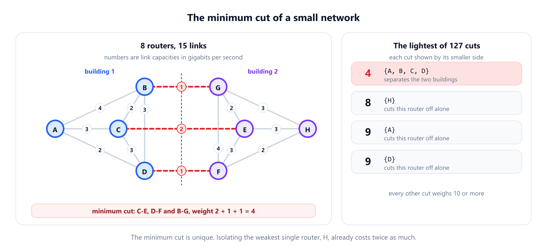
Cutting the three links between the buildings, C-E, D-F and B-G, costs 2 + 1 + 1 = 4 and splits the network in two. That is the minimum cut, and it is the only cut of weight 4. It is also the network's weakest point: the most traffic the two buildings can exchange is 4 gigabits per second, however the rest of the network is configured. The next cheapest cut isolates router H, at a cost of 8, the sum of its own links.
2. Two problems with the same name
"Minimum cut" names two related problems, and most confusion about the topic comes from mixing them up:
- Minimum s-t cut. Two vertices are given, a source
sand a sinkt, and the cut must separate them:sinS,toutside. This is the cut in the max-flow min-cut theorem of section 4. In the example, the minimum cut separatingAfromHis the building cut of weight 4, but the minimum cut separatingAfromBhas weight 9: with both in the same building, the cheapest option is to cut offAalone. - Global minimum cut. No vertices are given; the cut may separate any two groups. Its weight is the smallest of all s-t minimum cuts, and in an unweighted graph it equals the edge connectivity
λ(G), the fewest edges whose removal disconnects the graph. Sections 5 to 7 compute it.
A simple bound connects the two ideas. Cutting off a single vertex costs the sum of its link weights, its weighted degree, so the global minimum cut can never exceed the smallest degree. Hassler Whitney proved the unweighted version in 1932: vertex connectivity ≤ edge connectivity ≤ minimum degree. In the example the smallest weighted degree is 8, at H, and the minimum cut of 4 is well below it: the weak point is a bundle of links between two groups, not a single badly connected router. Without the weights the bound is tight here: every router has at least 3 links, and 3 links are the fewest that disconnect the network.
3. Why trying every cut does not scale
A graph with n vertices has 2n-1 - 1 cuts: each vertex other than a fixed first one goes to either side, and the split with everything on one side is not a cut. The example has 27 - 1 = 127, few enough to list.
from itertools import combinations

LINKS = [('A', 'B', 4), ('A', 'C', 3), ('A', 'D', 2), ('B', 'C', 2), ('B', 'D', 3), ('C', 'D', 3),
         ('E', 'F', 3), ('E', 'G', 2), ('E', 'H', 3), ('F', 'G', 4), ('F', 'H', 2), ('G', 'H', 3),
         ('C', 'E', 2), ('D', 'F', 1), ('B', 'G', 1)]

def cut_weight(side, links):
    """Total weight of the links with exactly one end in side."""
    return sum(w for u, v, w in links if (u in side) != (v in side))

def all_cuts(links):
    """Every split of the vertices into two nonempty sides, each counted once."""
    vertices = sorted({x for u, v, _ in links for x in (u, v)})
    first, rest = vertices[0], vertices[1:]
    for r in range(len(rest)):                 # side always contains the first vertex
        for others in combinations(rest, r):
            side = {first, *others}
            yield cut_weight(side, links), ''.join(sorted(side))

cuts = sorted(all_cuts(LINKS))
print(len(cuts), 'cuts')
# 127 cuts
for weight, side in cuts[:4]:
    print(weight, side)
# 4 ABCD
# 8 ABCDEFG
# 9 A
# 9 ABCEFGH
The count doubles with every vertex: 50 vertices already give more than 560 trillion cuts. The rest of this guide is about algorithms that find the minimum without looking at most of them. The guide to graph algorithm complexity explains why exponential growth like this rules out brute force.
4. Minimum s-t cuts from maximum flow
The max-flow min-cut theorem, stated by Lester Ford and Delbert Fulkerson in a RAND report of 1954 and published in 1956, the same year Peter Elias, Amiel Feinstein and Claude Shannon gave a different proof, says that the largest flow that can be sent from s to t equals the weight of the smallest cut separating them. One direction is easy: every unit of flow has to cross every s-t cut, so no flow can exceed any cut. The theorem's content is that the two always meet. The guide to network flow and the max-flow min-cut theorem proves it with augmenting paths.
The question had a military origin. In 1955 T. E. Harris and F. S. Ross of the RAND Corporation modelled the railways of the western Soviet Union and Eastern Europe as a network of 44 vertices and 105 edges, to find the cheapest set of lines to disrupt. They were interested in the cut more than the flow: their report marks a minimum cut of 163,000 tons as "the bottleneck". It was declassified only in 1999.
For computing cuts, the important part is how the cut falls out of a maximum flow. When no augmenting path from s to t remains, collect every vertex that s can still reach through edges with spare capacity, the residual graph. That set is the S side of a minimum cut, and the full edges leaving it are the cut. The program below runs the Edmonds-Karp algorithm, which always augments along a shortest path, and then reads off the cut. Each undirected link may carry flow in either direction.
from collections import deque

LINKS = [('A', 'B', 4), ('A', 'C', 3), ('A', 'D', 2), ('B', 'C', 2), ('B', 'D', 3), ('C', 'D', 3),
         ('E', 'F', 3), ('E', 'G', 2), ('E', 'H', 3), ('F', 'G', 4), ('F', 'H', 2), ('G', 'H', 3),
         ('C', 'E', 2), ('D', 'F', 1), ('B', 'G', 1)]

def min_st_cut(links, s, t):
    """Edmonds-Karp maximum flow, then the minimum s-t cut read off the residual graph."""
    cap = {}
    for u, v, w in links:                      # an undirected link carries flow either way
        cap.setdefault(u, {})[v] = cap.get(u, {}).get(v, 0) + w
        cap.setdefault(v, {})[u] = cap.get(v, {}).get(u, 0) + w
    flow = 0
    while True:
        parent, queue = {s: None}, deque([s])
        while queue and t not in parent:       # shortest augmenting path by BFS
            u = queue.popleft()
            for v, c in cap[u].items():
                if c > 0 and v not in parent:
                    parent[v] = u
                    queue.append(v)
        if t not in parent:
            break
        path, v = [], t
        while parent[v] is not None:
            path.append((parent[v], v))
            v = parent[v]
        push = min(cap[u][v] for u, v in path)
        for u, v in path:                      # use up capacity, open the reverse direction
            cap[u][v] -= push
            cap[v][u] += push
        flow += push
    side = set(parent)                         # still reachable from s in the residual graph
    cut = [(u, v, w) for u, v, w in links if (u in side) != (v in side)]
    return flow, ''.join(sorted(side)), cut

print(min_st_cut(LINKS, 'A', 'H'))
# (4, 'ABCD', [('C', 'E', 2), ('D', 'F', 1), ('B', 'G', 1)])
print(min_st_cut(LINKS, 'A', 'B'))
# (9, 'A', [('A', 'B', 4), ('A', 'C', 3), ('A', 'D', 2)])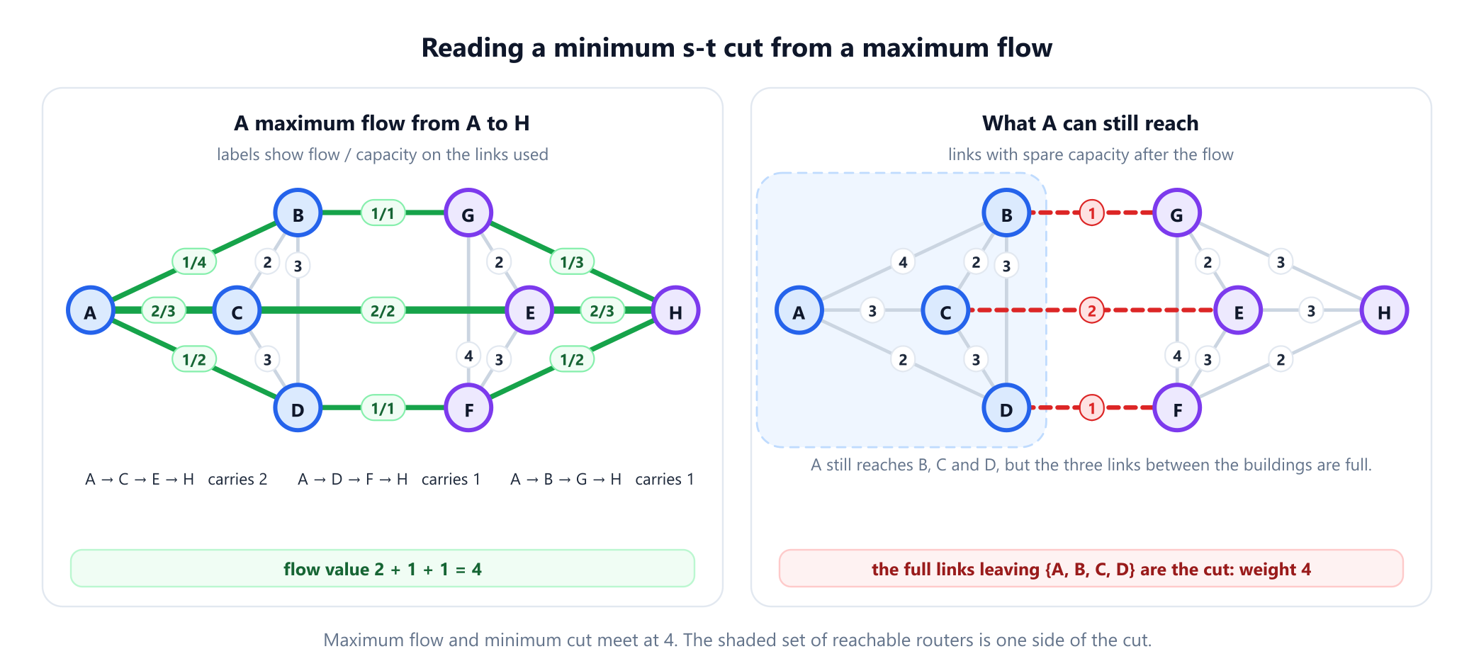
From A to H the maximum flow is 4, and it can be split into three paths carrying 2, 1 and 1 units. After that the three links between the buildings are full, A can still reach B, C and D but nothing beyond, and the cut is exactly the building cut. From A to B the flow is 9 and the cut isolates A. Edmonds-Karp runs in O(V E2) time; faster flow algorithms exist, but any correct one gives a minimum s-t cut this way.
For unweighted graphs the theorem has a famous combinatorial form, usually named after Karl Menger, whose theorem of 1927 is the version for vertices: the largest number of paths from u to v that share no edge equals the fewest edges whose removal separates u from v. This edge form of Menger's theorem follows from max-flow min-cut. In the example, ignoring weights, there are three edge-disjoint paths from A to H, and three links between the buildings.
5. Global minimum cuts with maximum flows
A global minimum cut separates some pair of vertices, so it is the smallest s-t cut over all pairs. Fewer pairs are enough. Fix any vertex s: whatever the minimum cut is, some vertex t lies on the other side of it, so the minimum over the n - 1 choices of t finds it. In the example, fixing s = A, the four runs with t in the other building all return 4.
Ralph Gomory and T. C. Hu showed in 1961 that n - 1 maximum flows reveal much more: they build a tree on the same vertices, now called the Gomory-Hu tree, in which the minimum cut between any two vertices equals the smallest edge weight on the tree path joining them. For the example the tree's seven edges carry the values 4, 8, 9, 9, 10, 10 and 10, so the value of every one of the 28 pairwise minimum cuts can be read off it, and the smallest edge, 4, is the global minimum cut.
Flow-based methods work for directed graphs too, and they are the right tool when the minimum cut between specific vertices matters. For the global minimum cut of an undirected graph, the next two algorithms are simpler and faster.
6. The Stoer-Wagner algorithm
In 1997, Mechthild Stoer and Frank Wagner published an algorithm that finds the global minimum cut of an undirected graph with nonnegative weights using no flows at all, building on earlier work by Hiroshi Nagamochi and Toshihide Ibaraki. It runs in n - 1 phases. Each phase does three things:
- Starting from any vertex, add vertices one at a time, always choosing the one most tightly connected to those already added: the largest total weight of links into the growing set. This ordering is known as a maximum adjacency search.
- When the last vertex
tis added, the weight of its links to everything else is the cut of the phase. A short argument shows it is a minimum cut separatingtfroms, the vertex added just before it. - Merge
sandtinto one vertex, adding the weights of parallel links, and start the next phase on the smaller graph.
Either the global minimum cut separates s from t, in which case this phase has found it, or it keeps them on the same side, in which case merging them loses nothing. After n - 1 phases the smallest cut of the phase is the answer.
LINKS = [('A', 'B', 4), ('A', 'C', 3), ('A', 'D', 2), ('B', 'C', 2), ('B', 'D', 3), ('C', 'D', 3),
         ('E', 'F', 3), ('E', 'G', 2), ('E', 'H', 3), ('F', 'G', 4), ('F', 'H', 2), ('G', 'H', 3),
         ('C', 'E', 2), ('D', 'F', 1), ('B', 'G', 1)]

def stoer_wagner(links):
    """Global minimum cut: n - 1 phases, each ending in a cut of the phase and one merge."""
    w = {}
    for u, v, c in links:
        w.setdefault(u, {})[v] = w.get(u, {}).get(v, 0) + c
        w.setdefault(v, {})[u] = w.get(v, {}).get(u, 0) + c
    groups = {v: v for v in w}                 # merged vertices remember what they contain
    best, phase = (float('inf'), ''), 0
    while len(w) > 1:
        phase += 1
        start = min(w)
        order, attached = [start], {v: w[start].get(v, 0) for v in w if v != start}
        while attached:                        # add the most tightly connected vertex next
            v = max(sorted(attached), key=attached.get)
            phase_cut = attached.pop(v)
            order.append(v)
            for x, c in w[v].items():
                if x in attached:
                    attached[x] += c
        s, t = order[-2], order[-1]
        side = ''.join(sorted(groups[t]))
        print(f'phase {phase}: cut of the phase {phase_cut:2}, side {side}')
        best = min(best, (phase_cut, side))
        for x, c in w.pop(t).items():          # merge t into s
            if x != s:
                w[s][x] = w[s].get(x, 0) + c
                w[x][s] = w[x].get(s, 0) + c
            del w[x][t]
        groups[s] += groups.pop(t)
    return best

print(stoer_wagner(LINKS))
# phase 1: cut of the phase  8, side H
# phase 2: cut of the phase 10, side F
# phase 3: cut of the phase 10, side FGH
# phase 4: cut of the phase  4, side EFGH
# phase 5: cut of the phase 10, side C
# phase 6: cut of the phase 10, side B
# phase 7: cut of the phase  9, side BCDEFGH
# (4, 'EFGH')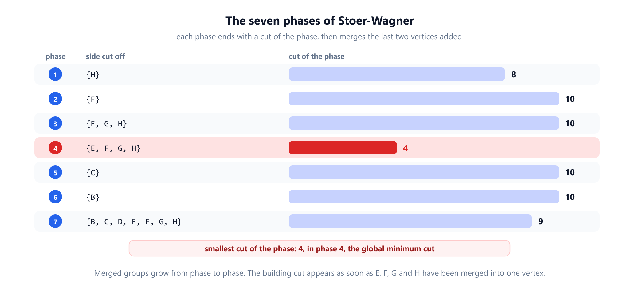
On the example, the first phase ends at H with a cut of 8, the cost of isolating it. As phases merge vertices, the groups grow: by phase 4 the last vertex added is the merged group E, F, G, H, and its cut of the phase is the building cut, 4. The remaining phases only find larger cuts. With a Fibonacci heap for the "most tightly connected" choice, each phase takes O(E + V log V) and the whole algorithm O(V E + V2 log V); the simple version above, which scans for the maximum, takes O(V3).
7. Karger's random contraction
David Karger's algorithm of 1993 is one of the most famous randomized algorithms. It is almost too simple to work:
- Pick a link at random, with probability proportional to its weight, and contract it: merge its two ends into one vertex, discarding the links between them.
- Repeat until only two merged vertices remain.
- The links between those two vertices form a cut. Report it.
One run can easily fail: if it ever contracts a link of the minimum cut, that cut is lost. The surprise is that it fails rarely enough. A minimum cut is light, so random choices tend to avoid its links, and Karger proved that a single run returns a given minimum cut with probability at least 2 / (n (n - 1)). Repeating the run and keeping the lightest cut drives the failure probability down as fast as you like.
import math, random

LINKS = [('A', 'B', 4), ('A', 'C', 3), ('A', 'D', 2), ('B', 'C', 2), ('B', 'D', 3), ('C', 'D', 3),
         ('E', 'F', 3), ('E', 'G', 2), ('E', 'H', 3), ('F', 'G', 4), ('F', 'H', 2), ('G', 'H', 3),
         ('C', 'E', 2), ('D', 'F', 1), ('B', 'G', 1)]

def contract(links, rnd):
    """One run of Karger's algorithm: merge the ends of random links until two groups remain."""
    group = {x: x for u, v, _ in links for x in (u, v)}
    def find(x):
        while group[x] != x:
            x = group[x]
        return x
    groups = len(group)
    while groups > 2:
        alive = [(u, v, w) for u, v, w in links if find(u) != find(v)]
        u, v, _ = rnd.choices(alive, weights=[w for *_, w in alive])[0]   # heavier links merge more often
        group[find(u)] = find(v)
        groups -= 1
    side = ''.join(sorted(x for x in group if find(x) == find('A')))
    return sum(w for u, v, w in links if find(u) != find(v)), side

rnd = random.Random(2026)
runs = [contract(LINKS, rnd) for _ in range(10_000)]
hits = sum(weight == 4 for weight, _ in runs)
print(f'minimum cut found in {hits} of 10,000 runs')
print(f'guaranteed at least 2 / (n (n - 1)) = {2 / (8 * 7):.4f} per run')
best_of_10 = [min(runs[i:i + 10]) for i in range(0, 10_000, 10)]
print(f'best of 10 runs is the minimum cut {sum(c[0] == 4 for c in best_of_10)} times out of 1,000')
print(f'runs needed for 99% with only the guarantee: {math.ceil(math.log(100) / -math.log(1 - 2 / 56))}')
# minimum cut found in 3228 of 10,000 runs
# guaranteed at least 2 / (n (n - 1)) = 0.0357 per run
# best of 10 runs is the minimum cut 978 times out of 1,000
# runs needed for 99% with only the guarantee: 127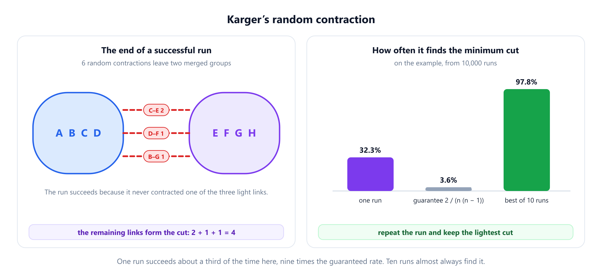
In 10,000 runs on the example, the minimum cut came out 3,228 times, about 32%, nine times the guaranteed 3.6%. Keeping the best of 10 runs found it in 978 of 1,000 trials. The guarantee is a worst case: relying on it alone, 127 runs would be needed for 99% confidence on 8 vertices. Karger's bound also has a striking consequence. Each minimum cut is found with probability at least 2 / (n (n - 1)), and these events cannot happen at the same time, so a graph can have at most n (n - 1) / 2 minimum cuts. A cycle on n vertices has exactly that many: removing any two of its edges is a minimum cut.
David Karger and Clifford Stein improved the method in 1996 by contracting only part of the way, then recursing on two copies, which finds a minimum cut with high probability in O(n2 log3 n) time. Karger later gave an algorithm that runs in nearly linear time in the number of edges.
8. Which algorithm to use
| Method | Finds | Time | Notes |
|---|---|---|---|
| Try every cut | Global or s-t | O(2n E) | Only for tiny graphs or checking other code |
| One maximum flow | Minimum s-t cut | That of the flow algorithm, O(V E2) for Edmonds-Karp | Works for directed graphs; the cut is read from the residual graph |
n - 1 maximum flows | Global, and with Gomory-Hu all pairs | n - 1 times one flow | The Gomory-Hu tree answers every pair's question at once |
| Stoer-Wagner | Global | O(V E + V2 log V) | Deterministic, no flows; undirected graphs, nonnegative weights |
| Karger, repeated | Global, with high probability | O(n2) per run with a simple implementation | Easy to code and to parallelise; can also list all minimum cuts |
| Karger-Stein | Global, with high probability | O(n2 log3 n) | Recursive contraction |
In practice: for the cut between two given vertices, run a maximum flow. For the global minimum cut of an undirected graph, Stoer-Wagner is the standard deterministic choice and is what libraries such as NetworkX implement. Karger's algorithm is the one to reach for when the graph is large, when the computation can be spread over many machines, or when you need every minimum cut rather than one.
9. Directed graphs and vertex cuts
In a directed graph, a cut (S, V \ S) counts only the arcs that go from S to the other side; arcs coming back do not help disconnect it. Stoer-Wagner and Karger's algorithm rely on symmetry and do not apply. The global minimum cut can still be found with maximum flows, from a fixed vertex to every other and back, and Jianxiu Hao and James Orlin showed in 1994 how to do it in about the time of a single flow computation.
Sometimes the question is which vertices to remove rather than which edges: the routers whose failure would split the network. The smallest such set gives the vertex connectivity, and a standard trick reduces it to edge cuts, by splitting each vertex into an "in" and an "out" copy joined by an edge of capacity 1. A single vertex whose removal disconnects the graph is an articulation point, and a single edge that does so is a bridge. Both can be found in linear time without flows, as the guide to connected components, bridges and articulation points explains.
10. Where minimum cuts are used
- Network reliability. The global minimum cut of a communication or power network is its weakest point: the fewest links, or least capacity, whose failure splits it. The minimum s-t cut is the bottleneck between two sites, as in the example.
- Image segmentation. Make each pixel a vertex joined to its neighbours, with heavy links between similar pixels, and add a source for "object" and a sink for "background". A minimum s-t cut separates object from background along the boundary that cuts the weakest links. D. M. Greig, B. T. Porteous and A. H. Seheult first used minimum cuts in image analysis in 1989, to restore noisy binary images, Zhenyu Wu and Richard Leahy applied them to segmentation in 1993, and Yuri Boykov's interactive graph cuts made the method a standard tool in computer vision.
- Clustering. A minimum cut splits a similarity graph where it is weakest. On its own it tends to cut off a few loosely attached points, which is why Jianbo Shi and Jitendra Malik introduced the normalized cut, which divides the cut weight by the size of each side.
- Project selection. Choosing projects that earn money but require costly prerequisites is a minimum cut problem in disguise: profitable projects hang from the source, costs from the sink, and prerequisites become infinite-capacity arcs. The guide to capital budgeting solves such a portfolio this way.
- Sports elimination. Whether a team can still finish first, given the remaining games, is a maximum flow question, and the minimum cut certifies a "no", as Benjamin Schwartz showed for baseball in 1966.
The opposite problem, the maximum cut, which asks for the split with as many crossing edges as possible, looks similar but is NP-hard. Minimising a cut is easy because it is dual to a flow; maximising one has no such structure.
11. Recent progress
Minimum cuts have seen some of the most striking recent advances in algorithms. In 2015, Ken-ichi Kawarabayashi and Mikkel Thorup found a deterministic algorithm for the global minimum cut of a simple unweighted graph that runs in near-linear time. In 2021, Jason Li extended deterministic almost-linear time to weighted graphs. And in 2022, Li Chen, Rasmus Kyng, Yang P. Liu, Richard Peng, Maximilian Probst Gutenberg and Sushant Sachdeva showed that maximum flow with integer capacities, and with it the minimum s-t cut, can be computed in almost-linear time m1 + o(1), a result that won the best paper award at FOCS 2022. These algorithms are not yet what practical software uses, but they settle how fast the problems can be solved in principle.
12. Common mistakes
| Mistake | Why it is wrong | Fix |
|---|---|---|
| Confusing the s-t and global minimum cut | From A to B the minimum cut is 9, but the global one is 4 | Ask whether two vertices must be separated |
| Taking the lightest vertex as the answer | The minimum degree is only an upper bound: 8 at H against a true minimum of 4 | Use Stoer-Wagner or Karger |
| Reading the cut from saturated edges alone | Full edges can lie inside one side; not every full edge is in the cut | Take the vertices reachable from s in the residual graph, then the edges leaving them |
| Running Stoer-Wagner on a directed graph | The algorithm assumes every link counts the same in both directions | Use maximum flows, or Hao-Orlin |
| Trusting a single Karger run | One run may succeed with probability as low as 2 / (n (n - 1)) | Repeat it and keep the lightest cut |
| Choosing links uniformly in a weighted graph | Karger's guarantee needs probability proportional to weight | Sample by weight, or treat weights as parallel links |
| Using plain minimum cuts for clustering | They tend to slice off a few loosely attached vertices | Use a balanced criterion such as the normalized cut |
| Expecting maximum cut to be just as easy | Maximum cut is NP-hard | Use approximation or heuristics for maximum cut |
13. Glossary
| Term | Meaning |
|---|---|
| Cut | A split of the vertices into two nonempty groups, or the set of edges crossing it |
| Cut weight (capacity) | The total weight of the edges crossing a cut |
| Minimum s-t cut | The lightest cut with s on one side and t on the other |
| Global minimum cut | The lightest cut of all, with no vertices prescribed |
| Edge connectivity | The fewest edges whose removal disconnects an unweighted graph |
| Vertex connectivity | The fewest vertices whose removal disconnects the graph |
| Residual graph | The links that still have spare capacity after a flow is sent |
| Max-flow min-cut theorem | The largest s-t flow equals the weight of the smallest s-t cut |
| Gomory-Hu tree | A tree that records the minimum cut between every pair of vertices |
| Cut of the phase | In Stoer-Wagner, the cut that isolates the last vertex added in a phase |
| Contraction | Merging the two ends of an edge into one vertex |
| Normalized cut | A cut weight divided by the sizes of the two sides, used for clustering |
14. Frequently asked questions
What is a minimum cut in a graph?
A cut splits the vertices of a graph into two nonempty groups, and its weight is the total weight of the edges that cross between them. A minimum cut is a cut of smallest weight: the cheapest set of edges whose removal disconnects the graph into two pieces. In an unweighted graph its size is the edge connectivity of the graph.
What is the difference between a minimum s-t cut and a global minimum cut?
A minimum s-t cut must separate two given vertices, a source s and a sink t, and is computed with a maximum flow. A global minimum cut may separate any two groups of vertices and is the smallest of all s-t minimum cuts. The two can differ a lot: two vertices in the same well-connected cluster can need a much heavier cut than the graph's weakest point.
How do you find the minimum cut from a maximum flow?
Compute a maximum flow from s to t. Then find every vertex that s can still reach through edges with spare capacity in the residual graph. Those vertices form one side of a minimum s-t cut, the full edges leaving them are the cut, and by the max-flow min-cut theorem its weight equals the value of the flow.
How does the Stoer-Wagner algorithm work?
Stoer-Wagner finds the global minimum cut of an undirected graph with nonnegative weights in n - 1 phases. Each phase adds vertices one at a time, always the one most tightly connected to those already added; the weight of the last vertex's links is a candidate cut, and the last two vertices are then merged. The smallest candidate is the minimum cut. It runs in O(VE + V squared log V) time with a Fibonacci heap.
How does Karger's algorithm work?
Karger's algorithm repeatedly picks a random edge, with probability proportional to its weight, and merges its two ends, until only two merged vertices remain; the edges between them form a cut. One run finds a given minimum cut with probability at least 2 / (n (n - 1)), so the algorithm is repeated many times and the lightest cut is kept. A consequence is that a graph has at most n (n - 1) / 2 minimum cuts.
Is the minimum cut problem NP-hard?
No. Both the minimum s-t cut and the global minimum cut can be found in polynomial time, with maximum flows, the Stoer-Wagner algorithm or Karger's randomized algorithm, and recent algorithms run in almost-linear time. The related maximum cut problem, which asks for the split with the most crossing edges, is NP-hard.
15. References
The theorems, algorithms and attributions above come from these sources, listed in chronological order.
- Menger, K. (1927). "Zur allgemeinen Kurventheorie." Fundamenta Mathematicae 10, 96 to 115.
- Whitney, H. (1932). "Congruent Graphs and the Connectivity of Graphs." American Journal of Mathematics 54(1), 150 to 168.
- Harris, T. E. and Ross, F. S. (1955). Fundamentals of a Method for Evaluating Rail Net Capacities. Research Memorandum RM-1573. Santa Monica: RAND Corporation.
- Elias, P., Feinstein, A. and Shannon, C. E. (1956). "A Note on the Maximum Flow Through a Network." IRE Transactions on Information Theory 2(4), 117 to 119.
- Ford, L. R. and Fulkerson, D. R. (1956). "Maximal Flow Through a Network." Canadian Journal of Mathematics 8, 399 to 404.
- Gomory, R. E. and Hu, T. C. (1961). "Multi-Terminal Network Flows." Journal of the Society for Industrial and Applied Mathematics 9(4), 551 to 570.
- Schwartz, B. L. (1966). "Possible Winners in Partially Completed Tournaments." SIAM Review 8(3), 302 to 308.
- Edmonds, J. and Karp, R. M. (1972). "Theoretical Improvements in Algorithmic Efficiency for Network Flow Problems." Journal of the ACM 19(2), 248 to 264.
- Greig, D. M., Porteous, B. T. and Seheult, A. H. (1989). "Exact Maximum A Posteriori Estimation for Binary Images." Journal of the Royal Statistical Society, Series B 51(2), 271 to 279.
- Nagamochi, H. and Ibaraki, T. (1992). "Computing Edge-Connectivity in Multigraphs and Capacitated Graphs." SIAM Journal on Discrete Mathematics 5(1), 54 to 66.
- Karger, D. R. (1993). "Global Min-cuts in RNC, and Other Ramifications of a Simple Min-cut Algorithm." In Proceedings of the 4th ACM-SIAM Symposium on Discrete Algorithms, 21 to 30.
- Wu, Z. and Leahy, R. (1993). "An Optimal Graph Theoretic Approach to Data Clustering: Theory and Its Application to Image Segmentation." IEEE Transactions on Pattern Analysis and Machine Intelligence 15(11), 1101 to 1113.
- Hao, J. and Orlin, J. B. (1994). "A Faster Algorithm for Finding the Minimum Cut in a Directed Graph." Journal of Algorithms 17(3), 424 to 446.
- Karger, D. R. and Stein, C. (1996). "A New Approach to the Minimum Cut Problem." Journal of the ACM 43(4), 601 to 640.
- Stoer, M. and Wagner, F. (1997). "A Simple Min-Cut Algorithm." Journal of the ACM 44(4), 585 to 591.
- Karger, D. R. (2000). "Minimum Cuts in Near-Linear Time." Journal of the ACM 47(1), 46 to 76.
- Shi, J. and Malik, J. (2000). "Normalized Cuts and Image Segmentation." IEEE Transactions on Pattern Analysis and Machine Intelligence 22(8), 888 to 905.
- Boykov, Y. and Jolly, M.-P. (2001). "Interactive Graph Cuts for Optimal Boundary and Region Segmentation of Objects in N-D Images." In Proceedings of the 8th IEEE International Conference on Computer Vision, 105 to 112.
- Schrijver, A. (2002). "On the History of the Transportation and Maximum Flow Problems." Mathematical Programming 91(3), 437 to 445.
- Kawarabayashi, K. and Thorup, M. (2015). "Deterministic Global Minimum Cut of a Simple Graph in Near-Linear Time." In Proceedings of the 47th ACM Symposium on Theory of Computing, 665 to 674.
- Li, J. (2021). "Deterministic Mincut in Almost-Linear Time." In Proceedings of the 53rd ACM Symposium on Theory of Computing, 384 to 395.
- Chen, L., Kyng, R., Liu, Y. P., Peng, R., Probst Gutenberg, M. and Sachdeva, S. (2022). "Maximum Flow and Minimum-Cost Flow in Almost-Linear Time." In Proceedings of the 63rd IEEE Symposium on Foundations of Computer Science, 612 to 623.
Find the cut yourself
Build the two-building network in the min cut calculator, choose A as the source and H as the sink, and watch the flow fill the three links between the buildings until the cut appears.
Open the calculator