
Table of Contents
- 1. Too much stock and too little both cost money
- 2. What stock costs
- 3. The distributor used throughout
- 4. How much to order: the economic order quantity
- 5. How much safety stock: service levels and supplier delays
- 6. Service level or fill rate?
- 7. The best policy, and what today's rule costs
- 8. Seasonal products: ordering as a shortest path
- 9. One warehouse or four? Risk pooling
- 10. Where in the supply chain to hold stock
- 11. Many products, one service target
- 12. What is easy, what is hard
- 13. What the model leaves out
- 14. From spreadsheet to inventory policy
- 15. Mistakes that quietly cost money
- 16. Frequently asked questions
- 17. References
1. Too much stock and too little both cost money
For most distributors, retailers and manufacturers, inventory is the largest asset on the balance sheet that nobody manages with a formula. Stock levels are set by rules of thumb such as "keep a month's supply" or "never run out of our best sellers", adjusted after every shortage and every cash squeeze. Both failure modes are expensive. Too much stock ties up cash, fills warehouses and risks obsolescence. Too little loses sales, triggers expensive expediting and damages customer relationships.
Inventory theory is where operations research began. Ford Harris published the economic order quantity in 1913, Kenneth Arrow, Theodore Harris and Jacob Marschak founded the modern theory of inventory under uncertainty in 1951, and Harvey Wagner and Thomson Whitin showed in 1958 that planning orders for changing demand is a shortest path problem. Edward Silver, David Pyke and Douglas Thomas's textbook and Sven Axsäter's Inventory Control cover the field as it is practised today.
This article takes one distributor and answers the question in its title seven ways: how much to order, how much safety stock to hold, which service measure to promise, how to plan a seasonal product, whether to run one warehouse or four, where in the supply chain to keep buffers, and how to set service levels across a product range. Every number was computed exactly from the model, not estimated.
2. What stock costs
Three costs decide how much stock a business should hold:
- Holding cost. Money tied up in stock could be earning a return elsewhere, and stock also needs space, insurance and handling, and some of it will be damaged or become obsolete. Holding cost is usually expressed as a percentage of the item's value per year. Here it is 25%, a common planning figure.
- Ordering cost. Each order carries a fixed cost for purchasing work, transport and receiving that does not depend on the quantity. Here it is $400 per order.
- Shortage cost. When a customer orders a drill that is not in stock, the order waits for the next delivery. Expedited shipping, discounts and lost goodwill are valued at $25 per drill short.
These figures are illustrative rather than taken from any particular company, but they are typical in structure. Holding cost pushes towards small, frequent orders and little safety stock; ordering cost pushes towards large, infrequent orders; shortage cost pushes towards more safety stock. The optimal policy balances all three.
3. The distributor used throughout
A tools distributor buys a best-selling cordless drill for $80 and sells it in four regions from one central warehouse. Weekly demand in each region varies around its average:
| Region | Average weekly demand | Standard deviation |
|---|---|---|
| North | 180 | 60 |
| South | 140 | 50 |
| East | 110 | 45 |
| West | 70 | 35 |
Total demand averages 500 drills a week, 26,000 a year. At a 25% holding rate each drill costs $20 a year to keep in stock. The supplier's lead time averages 2 weeks, but deliveries vary, with a standard deviation of half a week.
The distributor's current rule is simple: when stock falls to three weeks of demand, 1,500 drills, order a month's supply, 2,000 drills. The question is whether that rule is right.
4. How much to order: the economic order quantity
Start with the order size, ignoring uncertainty for a moment. Ordering more at a time means fewer orders a year but more stock on average, because stock falls from the order quantity to zero between deliveries and so averages half the order quantity. Harris's 1913 formula balances the two costs exactly:
EOQ = √(2 × annual demand × ordering cost / holding cost per unit per year)
For the drill that is √(2 × 26,000 × $400 / $20) = 1,020 drills, about two weeks of demand, at a yearly ordering and cycle-stock holding cost of $20,396.
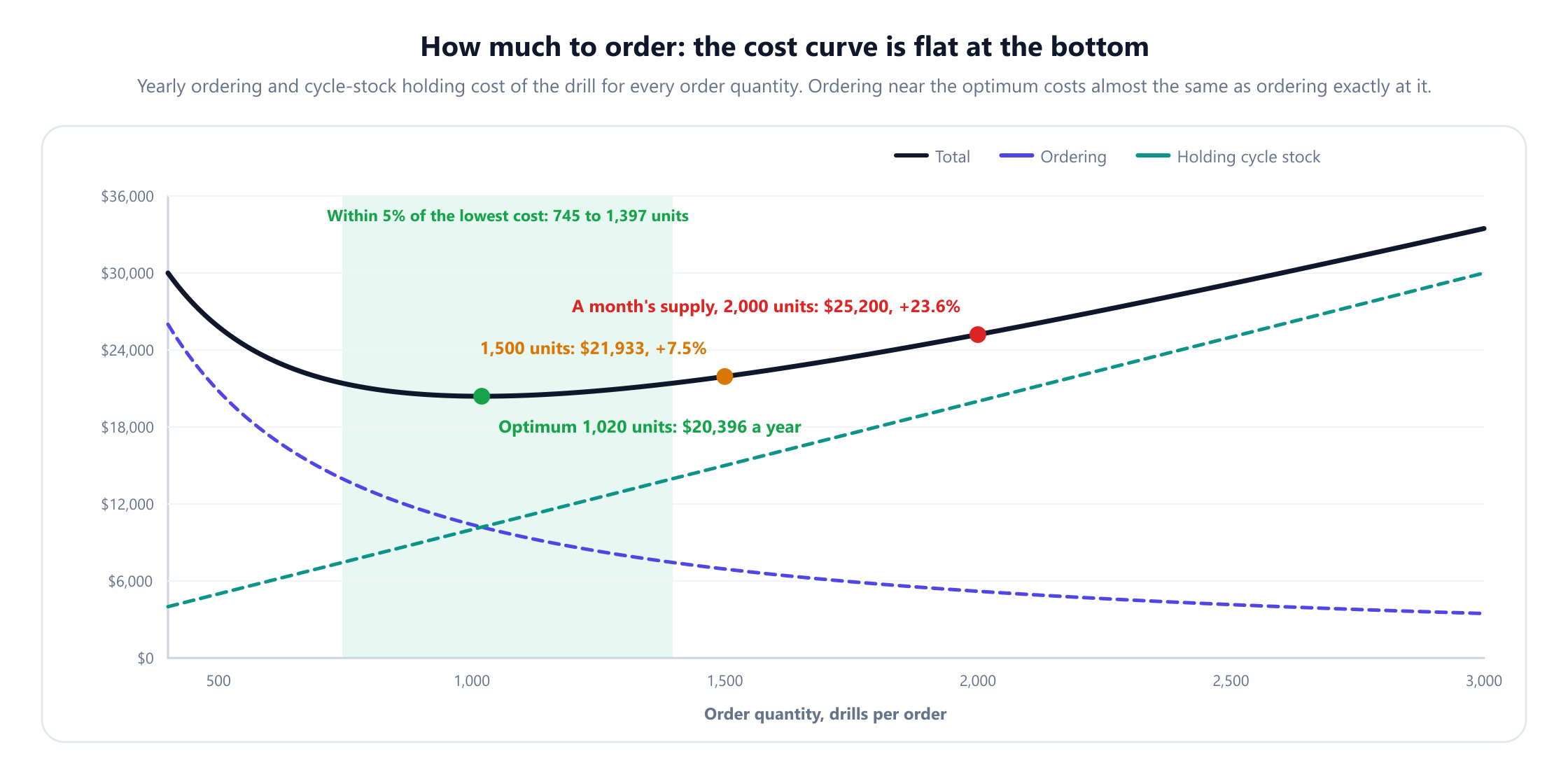
The curve's most useful property is its flat bottom. Any order quantity between 745 and 1,397 drills costs within 5% of the optimum, so rounding to a full pallet or a convenient truckload is harmless. Ordering 1,500 costs 7.5% more. Ordering a month's supply, 2,000 drills, costs $25,200, 23.6% more. The EOQ is robust to small errors in the cost estimates, which is why a formula from 1913 is still the starting point of every inventory system.
5. How much safety stock: service levels and supplier delays
Demand is not steady, and the supplier is not punctual. The risk of running out is concentrated in the time between placing an order and receiving it: if demand is high or the delivery is late, stock runs out before the order arrives. Safety stock is the extra stock held for that period, and the reorder point is expected demand during the lead time plus safety stock.
Expected demand during a 2-week lead time is 1,000 drills. Its variability combines two sources. Weekly demand varies independently across regions, and a late delivery adds a whole extra period of demand. The standard formula for the standard deviation of demand during the lead time is:
σ = √(lead time × weekly variance + average weekly demand² × lead time variance)
Here that is √(2 × 9,350 + 500² × 0.25) = √(18,700 + 62,500) = 285 drills. If the supplier were always exactly on time it would be only 137. Supplier delays account for 77% of the variance. Eppen and Martin (1988) also showed that the usual normal approximation can mislead when lead times vary, so this component deserves careful measurement.
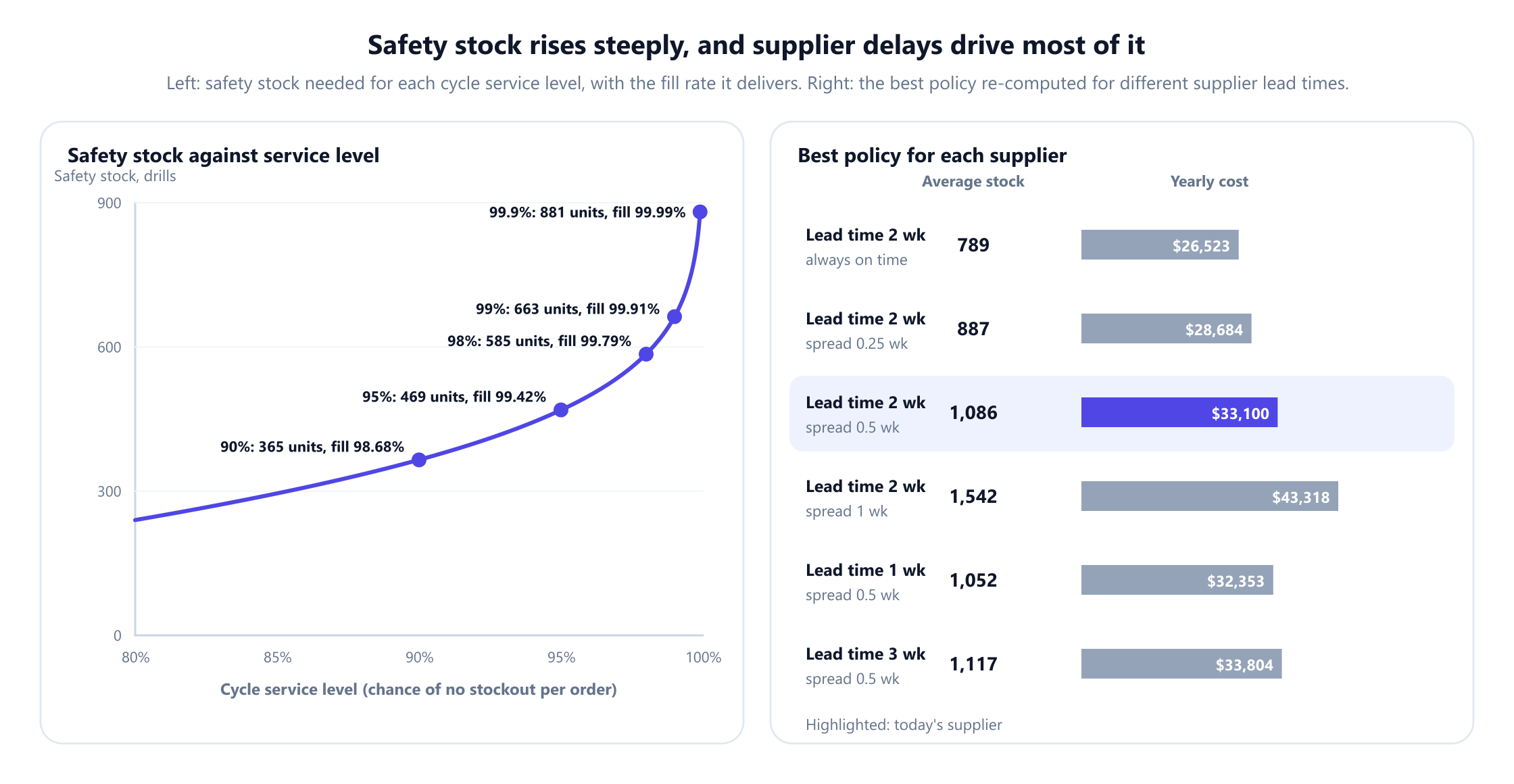
The cycle service level is the probability that stock does not run out before an order arrives. Assuming lead-time demand is roughly normal, safety stock is the service level's z-value times σ. With orders of 1,020 drills:
| Cycle service level | Safety stock | Yearly holding cost | Fill rate | Drills short per year | Yearly total cost |
|---|---|---|---|---|---|
| 90% | 365 | $17,500 | 98.68% | 344 | $36,305 |
| 95% | 469 | $19,580 | 99.42% | 151 | $33,561 |
| 98% | 585 | $21,900 | 99.79% | 53 | $33,432 |
| 99% | 663 | $23,460 | 99.91% | 25 | $34,271 |
| 99.9% | 881 | $27,820 | 99.99% | 2 | $38,066 |
The last step is the steepest: going from 99% to 99.9% needs 33% more safety stock to avoid about 23 shortages a year. The right-hand panel of the figure re-optimises the whole policy for different suppliers. A supplier who always delivered in exactly 2 weeks would cut average stock from 1,086 to 789 drills and yearly cost by $6,577. A supplier who delivered in 1 week, with the same unreliability, would save only $747. For this product, reliability is worth nearly nine times as much as speed, which is useful to know before negotiating with suppliers.
6. Service level or fill rate?
Service targets are often stated without saying what is measured, and the difference matters. The cycle service level counts replenishment cycles without a stockout. The fill rate counts the share of demand delivered from stock. A stockout late in a cycle may leave only a few customers waiting, so the fill rate is usually much higher than the cycle service level.
The expected shortage in a cycle is σ times the standard normal loss function of the z-value, and the fill rate is one minus that shortage divided by the order quantity. For the drill, a 95% cycle service level already delivers a 99.42% fill rate, and a 90% cycle service level delivers 98.68%. A manager who asks for "98% service" meaning fill rate, and receives a 98% cycle service level, gets 585 drills of safety stock, although 365 drills, a 90% cycle service level, would already have delivered 98.68%. Across a product range that confusion alone can inflate inventory by a large margin.
7. The best policy, and what today's rule costs
Order size and reorder point interact: larger orders mean fewer cycles, so fewer occasions to run out, so less safety stock is needed. Hadley and Whitin's 1963 method finds both together by alternating between the two formulas until they agree, and a final search over whole numbers confirms the optimum.
| Policy | Reorder point | Order quantity | Fill rate | Ordering | Holding | Shortages | Yearly total |
|---|---|---|---|---|---|---|---|
| EOQ, no safety stock | 1,000 | 1,020 | 88.85% | $10,196 | $10,200 | $72,444 | $92,840 |
| Current rule | 1,500 | 2,000 | 99.77% | $5,200 | $30,000 | $1,481 | $36,681 |
| EOQ, 99% service level | 1,663 | 1,020 | 99.91% | $10,196 | $23,460 | $615 | $34,271 |
| EOQ, 95% service level | 1,469 | 1,020 | 99.42% | $10,196 | $19,580 | $3,785 | $33,561 |
| Optimal | 1,516 | 1,139 | 99.65% | $9,131 | $21,710 | $2,259 | $33,100 |
The optimal policy reorders at 1,516 drills and orders 1,139 at a time, for $33,100 a year. The current rule costs $3,581 a year more for this one product, and holds about 415 more drills on average, around $33,000 of cash that could be used elsewhere. It does deliver a slightly higher fill rate, 99.77% against 99.65%, but at $25 per drill short that extra service is worth far less than the stock it takes.
The first row is the warning. Using the EOQ as a reorder rule with no safety stock runs out in half of all cycles, delivers only 88.9% of demand from stock, and costs $92,840 a year once shortages are counted. The EOQ answers how much to order, not when.
8. Seasonal products: ordering as a shortest path
The EOQ assumes steady demand. The distributor also sells patio heaters, whose demand swings with the seasons. Monthly forecasts are known, each order costs $900, and a heater held for a month costs $1.50. When should orders be placed, and how large should each be?
Wagner and Whitin (1958) proved that an optimal plan only orders when stock has run out, so every order covers the demand of a run of consecutive months. That turns planning into a shortest path problem. Draw nodes 0 to 12, where node t means "the first t months are covered", and an arc from i to j for an order placed in month i + 1 that covers months i + 1 to j. Its cost is $900 plus the holding cost of carrying the later months' heaters. Every plan is a path from node 0 to node 12, and the cheapest path is the best plan.
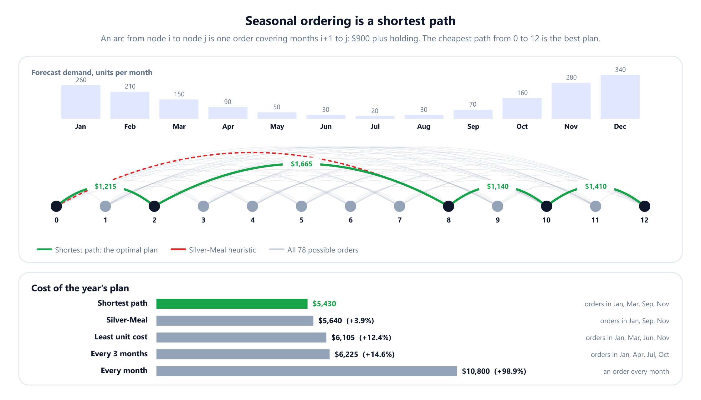
The graph is a directed acyclic graph with 78 arcs, so the shortest path takes one pass in order of the nodes, and Dijkstra's algorithm works too because every arc cost is positive. The optimal plan costs $5,430: order 470 heaters in January for January and February, 370 in March to cover the quiet months to August, 230 in September and 620 in November.
| Method | Orders placed in | Yearly cost | Above optimum |
|---|---|---|---|
| Order every month | Every month | $10,800 | +$5,370 |
| Order every 3 months | Jan, Apr, Jul, Oct | $6,225 | +$795 |
| Least unit cost | Jan, Mar, Jun, Nov | $6,105 | +$675 |
| Silver-Meal | Jan, Sep, Nov | $5,640 | +$210 |
| Shortest path | Jan, Mar, Sep, Nov | $5,430 | 0 |
The heuristics are all sensible. Ordering every 3 months uses the EOQ's average interval. Least unit cost extends each order while the cost per heater falls. The Silver-Meal heuristic (1973) extends each order while the cost per month falls, and it is the best of them here: its first order covers January to August, which saves an order but pays to store the spring and summer heaters from January onwards. It is still $210 above the optimum, and nothing in the heuristic says so. The shortest path is exact and just as fast to compute, and Wagelmans, van Hoesel and Kolen (1992) showed it can be solved in O(n log n) time for long horizons.
9. One warehouse or four? Risk pooling
The sales team proposes regional warehouses so customers get next-day delivery. Before weighing that benefit, price the inventory. Each regional warehouse would order drills directly from the supplier, with its own reorder point and order quantity.
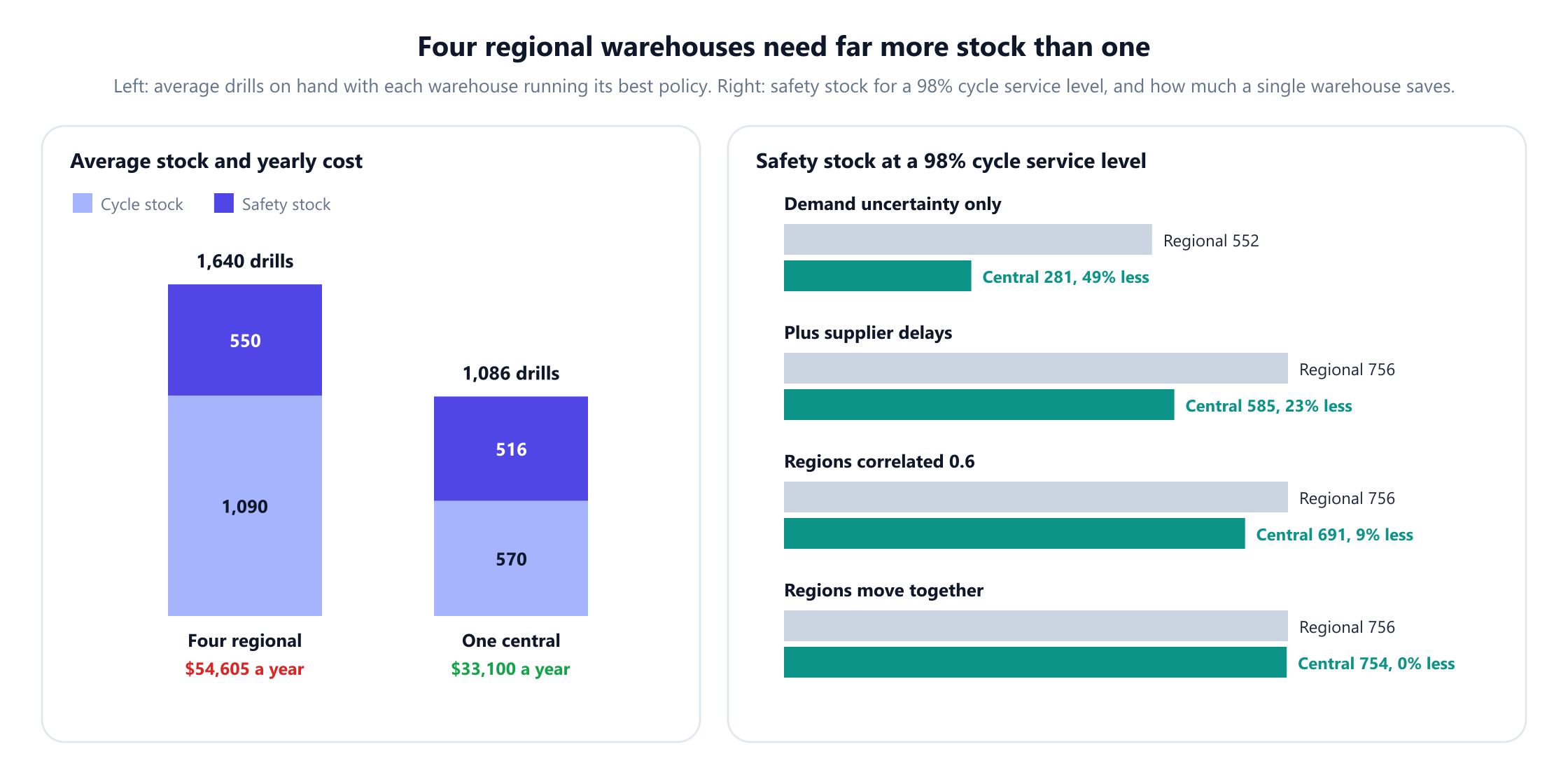
With every warehouse running its best policy, four regional warehouses cost $54,605 a year against $33,100 for one, $21,505 more, and hold about 555 more drills on average. Part of the difference is ordering: four warehouses place about twice as many orders in total, and each regional order is smaller, so cycle stock almost doubles from 570 to 1,090 drills.
The safety stock saving is the famous square-root law. If regional demands are independent, the standard deviation of total demand grows with the square root of the sum of the variances, not with the sum of the standard deviations. David Maister stated the law for inventory centralisation in 1976, and Gary Eppen proved the cost effect in 1979. At a 98% cycle service level, and counting demand uncertainty only, one warehouse needs 49% less safety stock than four.
Two things shrink the saving. Supplier delays hit all four warehouses at once, so pooling cannot cancel them out: with delays included, the saving falls to 23%. And when regions' demands rise and fall together, there is less to cancel: with a correlation of 0.6 between regions, the saving is 9%, and when regions move together it disappears. Pooling is most valuable for products with independent, noisy local demand and a reliable supplier, and least valuable for products driven by one national promotion calendar. The facility location guide covers the other side of this trade-off, transport cost and delivery distance.
10. Where in the supply chain to hold stock
So far the supplier has been a single lead time. In reality the drill passes through several stages, and safety stock could be held at any of them. The drill is made in a factory in 4 weeks, spends 5 weeks on a ship, takes 1 week to clear and ship out of the central warehouse, and 1 more week to reach a regional warehouse, where customers expect it to be in stock. Its value rises along the way, from $50 at the factory to $60 after shipping, $70 at the central warehouse and $80 in the regions.
The guaranteed service model, introduced by Kenneth Simpson in 1958 and made practical by Stephen Graves and Sean Willems in 2000, treats the supply chain as a graph. Each stage promises its customer a service time and holds enough safety stock to cover demand during its net replenishment time: the time its own supplier takes, plus its processing time, minus the time it promises downstream. A stage can hold a buffer, or it can hold nothing and pass its lead time downstream. Because safety stock grows with the square root of time, one buffer covering 10 weeks is much smaller than separate buffers for 4, 5 and 1 weeks.
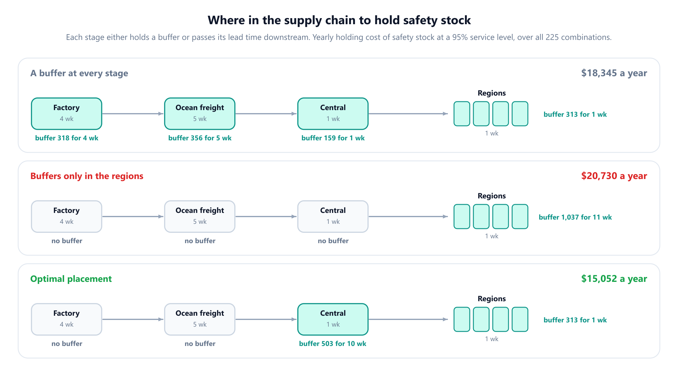
At a 95% service level, counting weekly demand variability only, all 225 combinations of service times can be checked. A buffer at every stage costs $18,345 a year to hold. Holding buffers only in the regions, where stock is most expensive and demand is split four ways, is worst at $20,730. The optimum holds no buffer at the factory or on the water, 503 drills at the central warehouse covering all 10 upstream weeks, and 313 drills in the regions for their final week, for $15,052 a year: 18% less than a buffer everywhere and 27% less than regional buffers only.
The central warehouse wins because it combines two advantages: it sees the pooled demand of all regions, and its drills are still cheaper than regional drills. For supply chains shaped as trees, Graves and Willems solve the problem with a dynamic programme over the graph, and Humair and Willems (2011) extended the approach to general acyclic networks. Andrew Clark and Herbert Scarf's 1960 work on serial systems is the foundation of the related stochastic-service models.
11. Many products, one service target
Real distributors manage thousands of products, and a common rule is to give them all the same service level, or to give the most valuable products the highest one. Consider six products that share a target: 98% of all units ordered delivered from stock.
| Product | Unit cost | Average weekly demand | Order quantity | Lead-time demand deviation | One service level | Optimal | Optimal, each at least 95% fill |
|---|---|---|---|---|---|---|---|
| Cordless drill | $80 | 500 | 1,020 | 285 | $14,640 | $12,080 | $12,880 |
| Battery pack | $25 | 900 | 2,448 | 210 | $3,375 | $6,075 | $4,400 |
| Charger | $30 | 300 | 1,290 | 120 | $2,310 | $2,610 | $1,080 |
| Circular saw | $150 | 120 | 365 | 90 | $8,700 | $0 | $6,600 |
| Blade pack | $6 | 700 | 4,406 | 260 | $1,002 | $2,304 | $1,896 |
| Laser level | $220 | 40 | 174 | 35 | $5,060 | $0 | $2,860 |
| Total safety stock investment | $35,087 | $23,069 | $29,716 |
Meeting the target with one cycle service level for every product requires 74%, and $35,087 of safety stock. But the target counts units, not dollars, and a unit of blade packs costs $6 while a laser level costs $220. The cheapest way to meet the target puts safety stock where each dollar prevents the most shortages. Because expected shortages fall with diminishing returns as safety stock rises, adding safety stock one unit at a time wherever it prevents the most shortages per dollar leads to the optimum, a result known as marginal analysis (Fox, 1966). The totals below are within one unit's cost of a mathematical lower bound on the best possible investment.
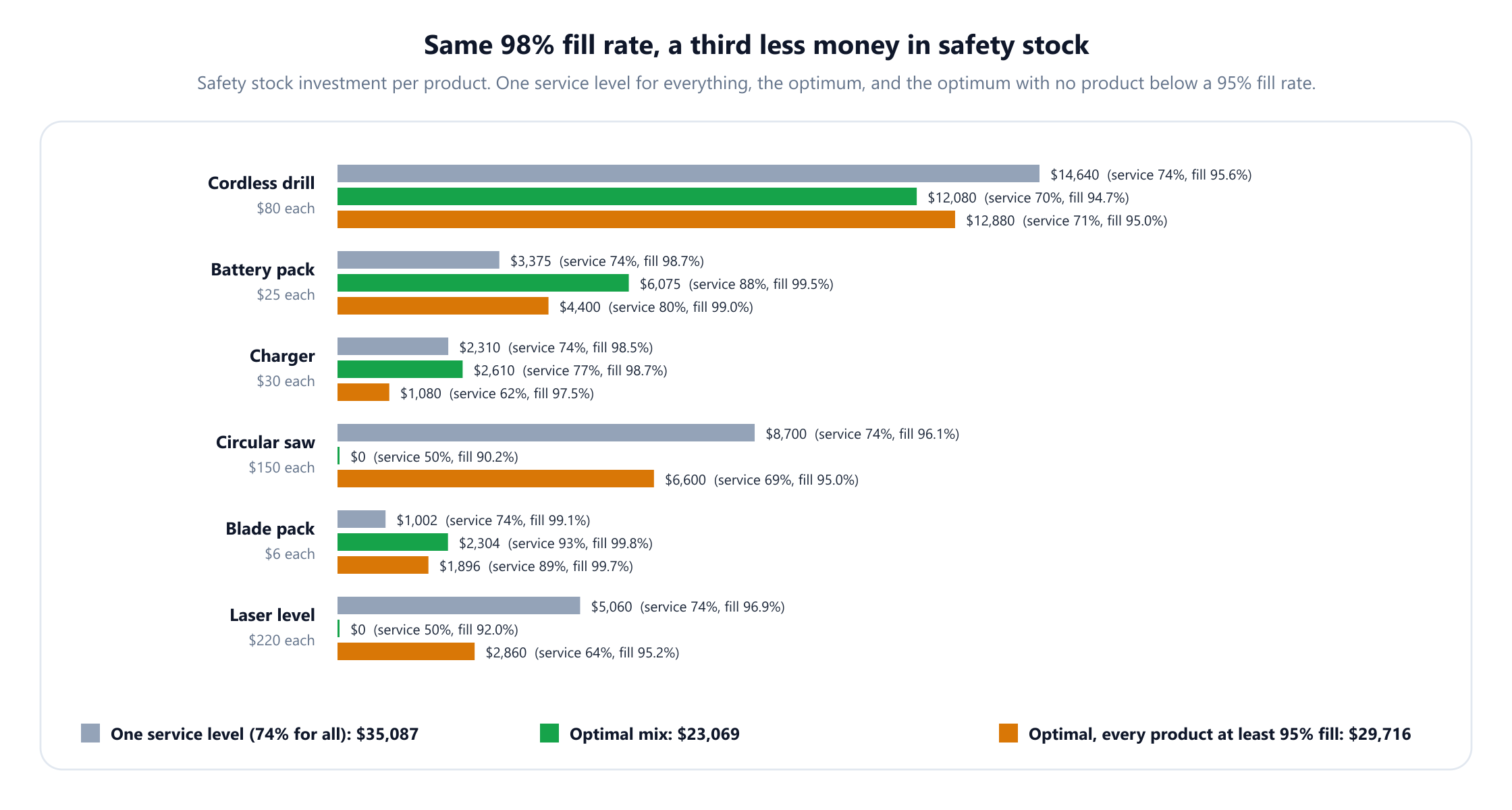
The optimum meets exactly the same 98% target with $23,069, 34% less. It raises blade packs to a 93% cycle service level and battery packs to 88%, and holds no safety stock at all for the circular saw and the laser level, whose fill rates fall to about 90% and 92%. That is often unacceptable commercially, so the last column adds a rule that no product may fall below a 95% fill rate. The optimum under that rule costs $29,716, still 15% less than one service level for all. Teunter, Babai and Syntetos (2010) proposed classifying products by a criterion that combines shortage cost, demand, holding cost and order quantity, and showed on real data sets that it achieves the same service at lower inventory cost than the usual classification by sales value.
12. What is easy, what is hard
| Problem | Method | Difficulty |
|---|---|---|
| Order quantity for steady demand | EOQ (Harris, 1913) | Closed-form formula |
| Safety stock for a service level | Normal distribution and loss function | Closed-form formula |
| Reorder point and order quantity together | Hadley and Whitin iteration | A few iterations |
| Uncapacitated lot sizing with changing demand | Shortest path (Wagner and Whitin, 1958) | Polynomial, O(n log n) |
| Lot sizing with limited capacity | Integer programming | NP-hard (Florian, Lenstra and Rinnooy Kan, 1980) |
| Serial supply chain with random demand | Echelon base-stock policies (Clark and Scarf, 1960) | Efficient stage-by-stage recursion |
| Safety stock placement on a tree | Dynamic programming (Graves and Willems, 2000) | Polynomial |
| Service levels across many products, one target | Marginal analysis or Lagrangian relaxation | Polynomial |
Compared with routing or scheduling, a surprising share of inventory optimisation is exactly solvable at scale. The hard parts are elsewhere: forecasting demand and its variability honestly, capturing capacity and minimum order constraints, and joining the separate models into one consistent policy. Paul Zipkin's Foundations of Inventory Management covers the theory behind each row.
13. What the model leaves out
- Forecast error. Safety stock should be based on the variability of forecast errors, not of raw demand, because a good forecast already explains part of the variation.
- Non-normal demand. Slow-moving and lumpy products are poorly described by the normal distribution. Poisson or negative binomial models, and Croston's method for intermittent demand, are more appropriate.
- Lost sales. The model assumes customers wait. In retail they often buy elsewhere, which changes the shortage cost and the formulas.
- Quantity discounts and minimum orders. Price breaks and supplier minimums change the order quantity, usually upwards.
- Shelf life and obsolescence. Perishable, fashion and technology products lose value, which calls for the newsvendor model of Arrow, Harris and Marschak rather than a steady reorder policy.
- Shared capacity. Warehouse space, working capital limits and truck sizes couple products together.
None of these changes the core picture: order quantity from the balance of ordering and holding cost, safety stock from lead-time variability and a correctly defined service target, and placement from where pooling and value are most favourable.
14. From spreadsheet to inventory policy
Measure the real inputs. Demand history by product and location is usually in the ERP system. Supplier lead times are too, as order and receipt dates, and the spread of actual lead times is often the biggest surprise. The holding cost rate belongs to finance, and it should include the cost of capital, not only storage.
Price today's rules. Compute the ordering, holding and shortage costs of the current reorder points and order quantities with the same model. For the drill that baseline showed $3,581 a year and 414 drills of excess stock. Repeated across a product range, that is the business case for a project.
Agree the service measure. Decide whether the target is a cycle service level, a unit fill rate or an order fill rate, and whether it applies per product or across the range. As section 11 showed, the choice changes the required investment by a third.
Work on the supply side too. Supplier reliability, shorter internal processing and pooling points often reduce inventory more than any formula. Most ERP and planning systems can hold reorder points and safety stocks computed elsewhere, and dedicated inventory optimisation tools add multi-echelon placement. Whatever the tool, re-compute parameters regularly, because demand and lead times drift. The supply chain optimisation guide shows how inventory fits with network flows and transport.
15. Mistakes that quietly cost money
- Ordering "a month's supply". For the drill it cost 23.6% more in ordering and cycle stock than the economic order quantity.
- Using the EOQ without safety stock. The drill ran out in half of all cycles, and the year cost $92,840.
- Ignoring supplier delays. They caused 77% of the drill's lead-time demand variance, and removing them was worth $6,577 a year, nearly nine times the value of a faster supplier.
- Confusing service level with fill rate. A 95% cycle service level already delivered a 99.42% fill rate.
- Trusting a lot-sizing heuristic. Silver-Meal was $210 above the shortest path for patio heaters, and gave no sign of it.
- Opening warehouses without pricing the stock. Four regional warehouses cost $21,505 a year more in inventory costs for the drill alone.
- Buffering at every stage, or only near the customer. The best placement was 18% cheaper than buffers everywhere and 27% cheaper than regional buffers only.
- One service level for every product. The same 98% fill rate needed $35,087 of safety stock one way and $23,069 the other.
16. Frequently asked questions
What is inventory optimization?
+
It is setting order quantities, reorder points and safety stocks so that a target level of customer service is met at the lowest total cost of ordering, holding stock and shortages. It uses demand and lead-time data, cost parameters and models such as the economic order quantity, service level formulas, lot sizing and multi-echelon safety stock placement, instead of rules of thumb such as holding a fixed number of weeks of supply.
How do you calculate safety stock?
+
Safety stock is the z-value of the chosen cycle service level multiplied by the standard deviation of demand during the lead time. When both demand and lead time vary, that standard deviation is the square root of the lead time times the variance of demand per period plus the square of average demand times the variance of the lead time. In the article's example, a 95% cycle service level needed 469 drills of safety stock.
What is the difference between service level and fill rate?
+
The cycle service level is the probability that stock does not run out during a replenishment cycle. The fill rate is the share of demand delivered immediately from stock. Because a stockout often affects only a few units at the end of a cycle, the fill rate is usually much higher: in the example, a 95% cycle service level delivered a 99.42% fill rate. Setting targets without saying which is meant leads to excess inventory.
Is the economic order quantity still useful?
+
Yes, as a starting point for order sizes. Its total cost curve is flat near the optimum, so rounding to pallets or truckloads costs little: in the example, any quantity between 745 and 1,397 units cost within 5% of the minimum. It does not set reorder points or safety stock, it assumes steady demand, and it should be adjusted for quantity discounts, minimum orders and capacity limits.
What is the Wagner-Whitin algorithm?
+
It finds the cheapest schedule of orders for a product with known but changing demand, fixed ordering costs and holding costs. Because an optimal plan orders only when stock runs out, each order covers a run of consecutive periods, and the problem becomes a shortest path through a directed acyclic graph whose arcs are possible orders. In the example it beat the Silver-Meal heuristic by $210 over a year.
Does centralizing inventory always reduce stock?
+
It reduces cycle stock and ordering costs, and it reduces safety stock when local demands are independent, following the square-root law. The safety stock benefit shrinks when uncertainty is shared: in the example, one warehouse needed 49% less safety stock than four for demand uncertainty alone, 23% less once supplier delays were included, and none less when regional demands moved together. Transport costs and delivery times must be weighed against the saving.
Should expensive products have higher service levels?
+
Not if the target is a fill rate across units. Safety stock on cheap products prevents more shortages per dollar, so the cost-optimal allocation gives cheap, fast-moving products higher service and expensive ones lower service. In the example this met the same 98% fill rate with $23,069 of safety stock instead of $35,087, and $29,716 when every product was kept at a 95% fill rate or better.
17. References
The foundational papers, surveys and books behind the methods in this article, in chronological order.
- Harris, F. W. (1913). “How many parts to make at once.” Factory, The Magazine of Management, 10(2), 135–136, 152.
- Arrow, K. J., Harris, T. and Marschak, J. (1951). “Optimal inventory policy.” Econometrica, 19(3), 250–272.
- Simpson, K. F. (1958). “In-process inventories.” Operations Research, 6(6), 863–873.
- Wagner, H. M. and Whitin, T. M. (1958). “Dynamic version of the economic lot size model.” Management Science, 5(1), 89–96.
- Clark, A. J. and Scarf, H. (1960). “Optimal policies for a multi-echelon inventory problem.” Management Science, 6(4), 475–490.
- Hadley, G. and Whitin, T. M. (1963). Analysis of Inventory Systems. Englewood Cliffs: Prentice-Hall.
- Fox, B. (1966). “Discrete optimization via marginal analysis.” Management Science, 13(3), 210–216.
- Silver, E. A. and Meal, H. C. (1973). “A heuristic for selecting lot size quantities for the case of a deterministic time-varying demand rate and discrete opportunities for replenishment.” Production and Inventory Management, 14(2), 64–74.
- Maister, D. H. (1976). “Centralisation of inventories and the ‘square root law’.” International Journal of Physical Distribution, 6(3), 124–134.
- Eppen, G. D. (1979). “Effects of centralization on expected costs in a multi-location newsboy problem.” Management Science, 25(5), 498–501.
- Florian, M., Lenstra, J. K. and Rinnooy Kan, A. H. G. (1980). “Deterministic production planning: algorithms and complexity.” Management Science, 26(7), 669–679.
- Eppen, G. D. and Martin, R. K. (1988). “Determining safety stock in the presence of stochastic lead time and demand.” Management Science, 34(11), 1380–1390.
- Wagelmans, A., van Hoesel, S. and Kolen, A. (1992). “Economic lot-sizing: an O(n log n) algorithm that runs in linear time in the Wagner-Whitin case.” Operations Research, 40(Supplement 1), S145–S156.
- Graves, S. C. and Willems, S. P. (2000). “Optimizing strategic safety stock placement in supply chains.” Manufacturing & Service Operations Management, 2(1), 68–83.
- Zipkin, P. H. (2000). Foundations of Inventory Management. Boston: McGraw-Hill.
- Teunter, R. H., Babai, M. Z. and Syntetos, A. A. (2010). “ABC classification: service levels and inventory costs.” Production and Operations Management, 19(3), 343–352.
- Humair, S. and Willems, S. P. (2011). “Optimizing strategic safety stock placement in general acyclic networks.” Operations Research, 59(3), 781–787.
- Axsäter, S. (2015). Inventory Control, 3rd edition. Cham: Springer.
- Silver, E. A., Pyke, D. F. and Thomas, D. J. (2017). Inventory and Production Management in Supply Chains, 4th edition. Boca Raton: CRC Press.