
Table of Contents
- 1. Why location is the decision that fixes every later cost
- 2. What a distribution network costs
- 3. Step one: the region as a graph
- 4. The centre of gravity method
- 5. Greedy siting: add, drop and swap
- 6. The exact answer
- 7. Hakimi's theorem: medians sit at towns, centres may not
- 8. How many warehouses?
- 9. Pricing a service promise
- 10. Single sourcing
- 11. Losing a warehouse
- 12. What is easy, what is hard
- 13. What the model leaves out
- 14. Running a location study
- 15. Mistakes that quietly cost money
- 16. Frequently asked questions
- 17. References
1. Why location is the decision that fixes every later cost
Most logistics decisions can be changed next week: a delivery route, a shift pattern, a carrier. Where a warehouse stands cannot. A lease runs for years, a building is fitted out once, and every delivery made from it afterwards starts from that address. Choose a site in the wrong place and the business pays the extra kilometres on every order, for as long as the site stays open, and no amount of clever routing gets them back.
That is why facility location is one of the oldest and most studied problems in operations research. Alfred Weber asked in 1909 where a plant should stand to minimise the weighted distance to its suppliers and customers. In 1963 Kuehn and Hamburger published a computer heuristic for locating warehouses, and in 1964 Louis Hakimi recast the question on a network, proving the results that still justify how location studies are run. Reviews by Owen and Daskin (1998) and by Melo, Nickel and Saldanha-da-Gama (2009) trace how the problem became central to supply chain design.
The problem is naturally a graph problem. Towns are vertices, roads are weighted edges, and what matters is the length of the shortest path from a warehouse to each customer, not the distance on a map. Once the region is written down that way, the questions become precise: which sites to open, how many, which customers each serves, and what a promise to customers costs.
This article takes one realistic region, 14 towns, a road network with winding hill roads, and six candidate warehouse sites, and decides where to build using four common methods. The last is not a heuristic: it checks every possible combination of sites, so each method can be measured against a proven optimum. All the numbers below were computed by solving the model, not estimated.
2. What a distribution network costs
A warehouse network has two kinds of cost, and they pull in opposite directions.
- Fixed cost per site: lease or depreciation, staff, equipment and systems, paid every year whether the site ships a lot or a little.
- Delivery cost: paid per tonne and per kilometre on every delivery from a warehouse to a customer. In this article it is $0.08 per tonne-kilometre.
Open more warehouses and the fixed cost rises while the average delivery gets shorter. Open fewer and the reverse happens. The best network is where the two balance, and because sites also differ in cost and capacity, where that balance falls depends on exactly which sites are chosen.
The distributor in this article delivers 147,000 tonnes a year to 14 towns and can choose among six candidate sites:
| Candidate site | Fixed cost per year | Capacity, tonnes per year |
|---|---|---|
| Bexley | $120,000 | 75,000 |
| Carlow | $130,000 | 85,000 |
| Glenby | $120,000 | 85,000 |
| Hartley | $110,000 | 75,000 |
| Kendal | $100,000 | 70,000 |
| Marlow | $100,000 | 85,000 |
These figures are illustrative rather than taken from any real company, but the structure is typical, and the conclusions depend on the structure. One consequence is visible immediately: no single site can carry 147,000 tonnes, because the largest holds 85,000. Whatever the answer is, it involves at least two warehouses.
3. Step one: the region as a graph
The region is a weighted, undirected graph: 14 towns as vertices and 26 roads as edges, each labelled with its length in kilometres. The number that drives every cost is the road distance between a warehouse and a town, the length of the shortest path between them, computed for all pairs with the Floyd-Warshall algorithm or by running Dijkstra's algorithm from every town.
| Town | Tonnes per year | Town | Tonnes per year |
|---|---|---|---|
| Ashford | 8,000 | Hartley | 11,000 |
| Bexley | 12,000 | Irvine | 13,000 |
| Carlow | 15,000 | Jarrow | 5,000 |
| Dunmore | 9,000 | Kendal | 9,000 |
| Elton | 6,000 | Lisle | 12,000 |
| Farnham | 10,000 | Marlow | 16,000 |
| Glenby | 14,000 | Norton | 7,000 |
Road distance and map distance disagree more than intuition suggests. Across all pairs of towns in this region, the road is on average 28% longer than the straight line. Two hill roads make the gap dramatic in places: Carlow and Hartley are 49 km apart on the map but 94 km apart by road, 1.91 times as far, and the shortest drive from Glenby to Lisle is 112 km although the two towns are 69 km apart as the crow flies. Any method that measures straight lines will think those towns are neighbours. As section 4 shows, that mistake is expensive.
4. The centre of gravity method
The most widely taught quick method is the centre of gravity. Plot every customer on a map, weight each by its volume, and find the point that minimises the total weighted straight-line distance. That is Weber's problem, and Endre Weiszfeld gave the standard algorithm for it in 1937: start at the weighted average position and repeatedly move to a weighted average in which nearer customers count more, until the point stops moving. For several warehouses, Leon Cooper's 1964 location-allocation method alternates two steps: assign each customer to its nearest centre, then move each centre to the Weiszfeld point of its customers.
Told that three warehouses are needed, the method produces three points, and the planner opens the candidate site nearest each one.
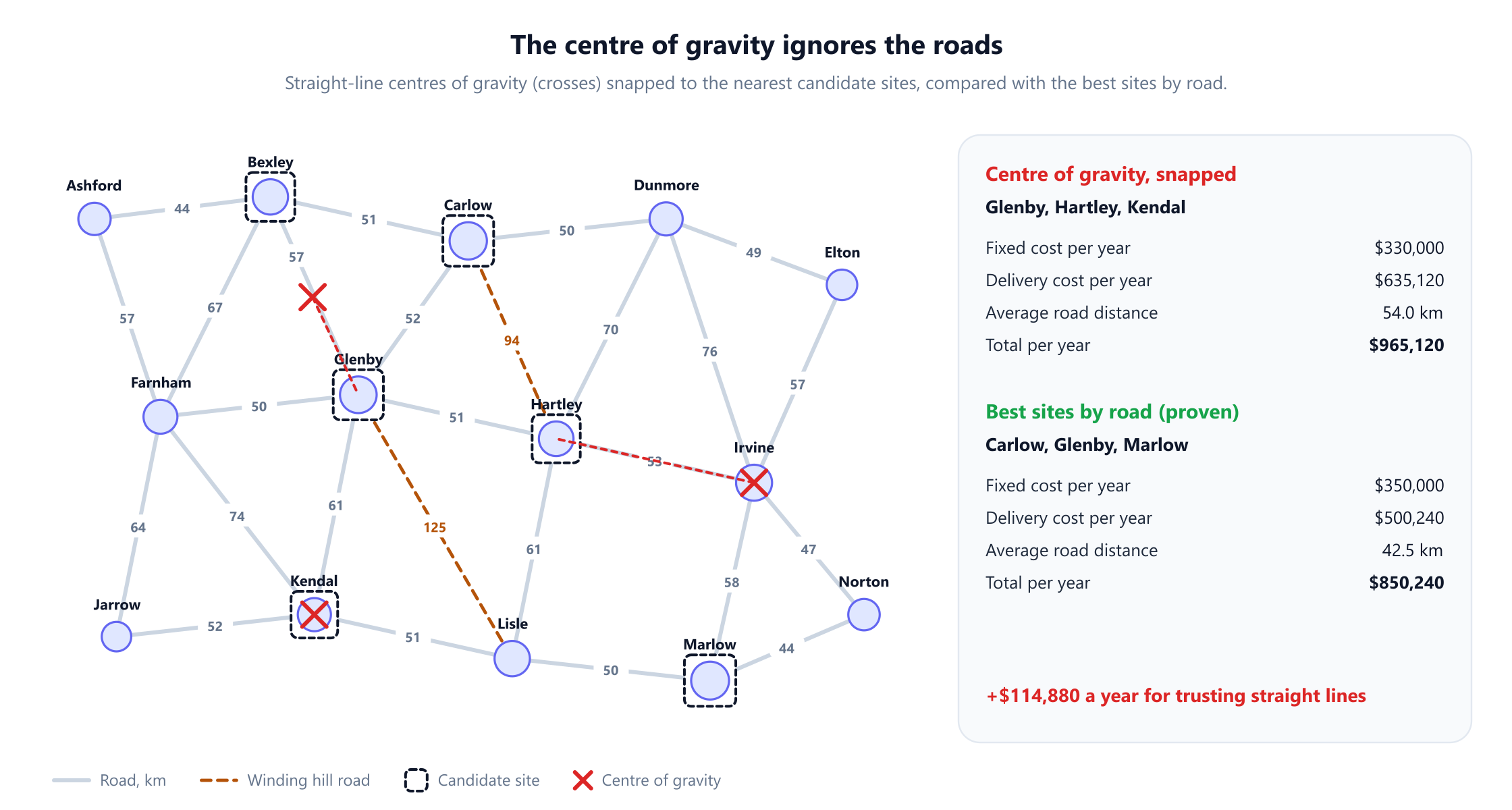
The three points land in revealing places. The western centre falls on the road between Bexley and Glenby and snaps to Glenby. The southern centre, serving Jarrow, Kendal and Lisle, lands exactly on Kendal. The eastern centre, serving six towns from Dunmore to Norton, lands exactly on Irvine, which is not a candidate site, and snaps to the nearest one, Hartley.
Priced on real roads, the plan Glenby, Hartley and Kendal costs $965,120 a year, with an average delivery of 54.0 km. The worst consequence is at Marlow, the largest customer at 16,000 tonnes a year. By straight line Marlow belongs with the eastern towns, but the snapped eastern warehouse at Hartley is 111 km away by road, so Marlow ends up served from Kendal, 101 km away. The best network, found in section 6, costs $850,240. Trusting straight lines costs $114,880 a year, 13.5% more.
Two separate errors compound here. The method measures the wrong distance, and it chooses points that are not sites, so the final snapping step is a guess. Neither error is visible on the centre of gravity's own terms: on the map, its answer looks sensible.
5. Greedy siting: add, drop and swap
Three classic heuristics work directly with the candidate sites and road distances.
ADD. Kuehn and Hamburger's 1963 method starts with no warehouses, opens the single site with the lowest total cost, and then keeps adding whichever site lowers the total most, until no addition helps. As published it ignores capacity while choosing, sending every town to its nearest open site.
Its first choice is Hartley. On its own, Hartley would cost $1,122,880 a year against $1,129,280 for Glenby: Glenby's central position saves $3,600 of delivery, but Hartley's fixed cost is $10,000 lower, so Hartley wins by $6,400. Hartley alone cannot carry the volume, so ADD keeps going: adding Glenby brings the cost to $955,840, adding Marlow brings it to $871,840, and no fourth site helps. The final plan, Glenby, Hartley and Marlow, costs $871,840, which is $21,600 a year above the optimum. The weakness is structural: ADD never reconsiders its first choice, and a decision made when one warehouse was on the map is the wrong one when there are three.
DROP. Feldman, Lehrer and Ray's 1966 method works the other way: open every site and keep closing the one whose closure saves most. With all six open the network costs $980,240. Closing Hartley gives $920,320, closing Bexley $881,920, closing Kendal $850,240, and closing any fourth site would raise the cost. On this region DROP finds the optimum. That is not a guarantee; both greedy methods can stop at a plan that no single addition or closure improves, while a better combination exists.
Swap. Teitz and Bart's 1968 interchange method takes any starting plan and exchanges one open site for one closed site whenever that lowers the cost. Starting from the centre of gravity's plan, it swaps Hartley for Marlow ($869,040) and then Kendal for Carlow, reaching $850,240 in two moves. Starting a local improvement method from a quick estimate is how most practical location software works.
6. The exact answer
Six candidate sites give 26 - 1 = 63 non-empty combinations, few enough to check every one. For each combination the remaining question is how to ship each town's volume from the open sites at least cost without exceeding any capacity. That is the transportation problem, posed by Hitchcock in 1941, and it is a minimum cost flow on a graph from warehouses to towns, solved exactly in polynomial time; the network flow guide covers the underlying theory.
Capacity rules some combinations out immediately. None of the six single sites can carry 147,000 tonnes, and 2 of the 15 pairs cannot either. The remaining 55 combinations are solved and compared.
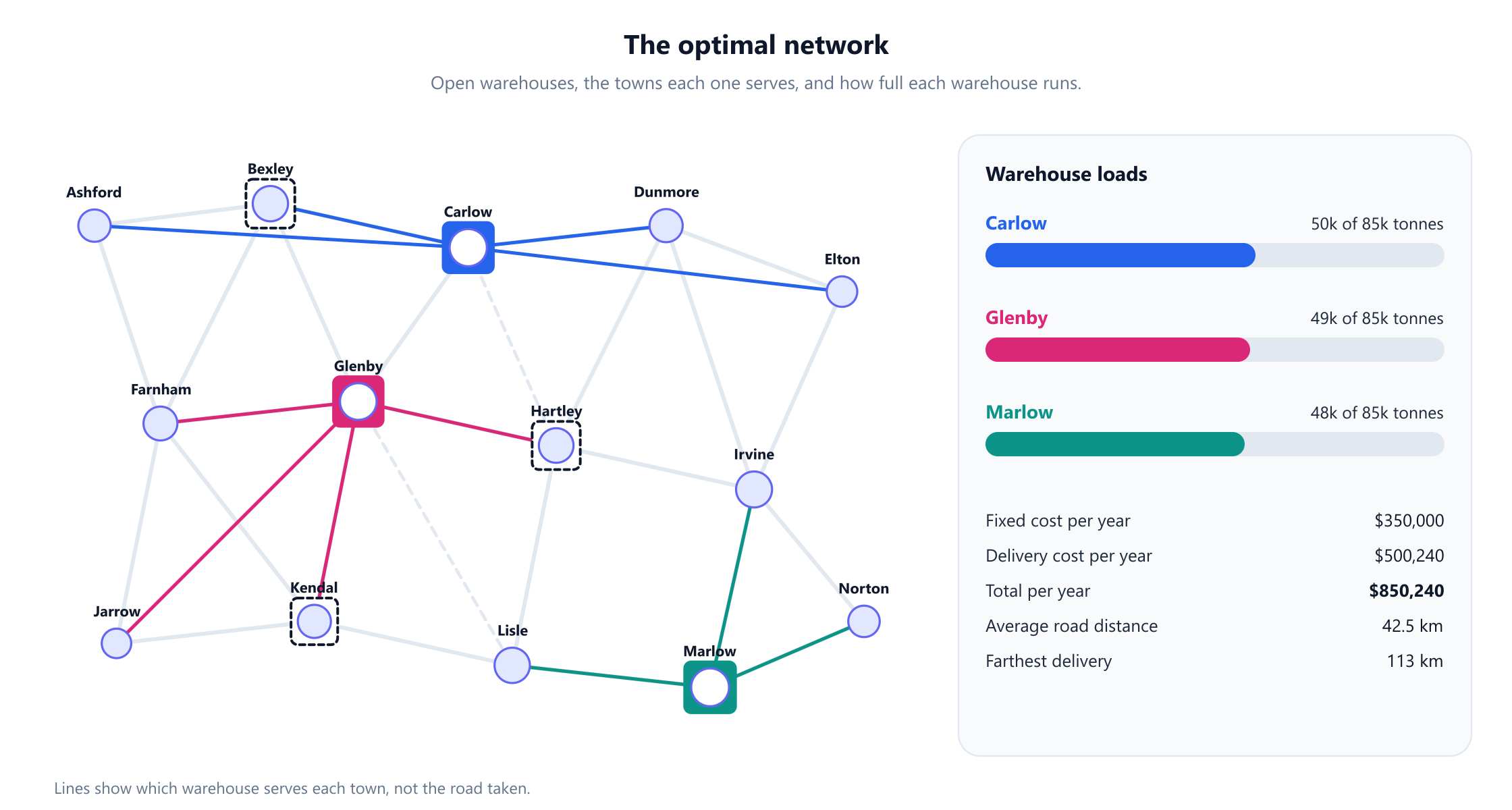
The optimum opens Carlow, Glenby and Marlow for $850,240 a year: $350,000 of fixed cost and $500,240 of delivery, an average of 42.5 km per tonne and $3.40 of delivery per tonne. The three warehouses run at 50,000, 49,000 and 48,000 tonnes against 85,000 of capacity each. Every town happens to be served entirely from one warehouse, and Carlow earns its place despite the highest fixed cost of the six by covering the northern towns that no other site reaches cheaply.
| Method | Sites opened | Fixed cost | Delivery cost | Total per year | Above optimum |
|---|---|---|---|---|---|
| Centre of gravity | Glenby, Hartley, Kendal | $330,000 | $635,120 | $965,120 | +$114,880 |
| Greedy ADD | Glenby, Hartley, Marlow | $330,000 | $541,840 | $871,840 | +$21,600 |
| Greedy DROP | Carlow, Glenby, Marlow | $350,000 | $500,240 | $850,240 | 0 |
| Centre of gravity, then swaps | Carlow, Glenby, Marlow | $350,000 | $500,240 | $850,240 | 0 |
| Proven optimum | Carlow, Glenby, Marlow | $350,000 | $500,240 | $850,240 | 0 |
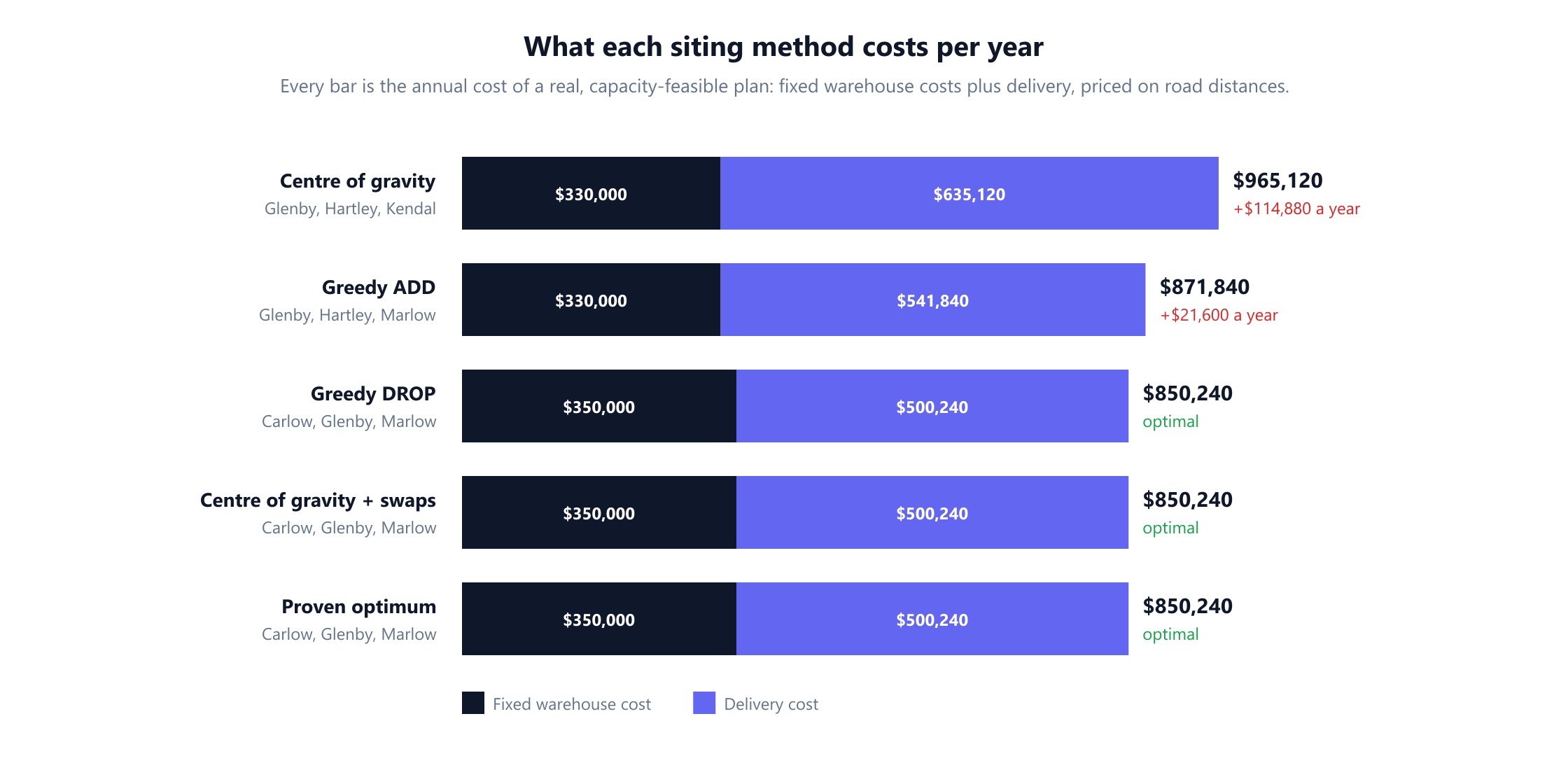
Note what the two worse plans have in common: both spend $20,000 a year less on fixed cost than the optimum, and both lose far more on delivery. The cheapest set of buildings is not the cheapest network. Over a ten-year lease, the centre of gravity's plan would cost about $1.15 million more than the optimum and ADD's about $216,000 more, before any growth in volume.
Checking every combination only works for a handful of sites. With 30 candidates there are more than a billion combinations, so real studies formulate the problem as a mixed integer programme, with a yes-or-no variable for each site and flow variables for each assignment, the formulation Balinski gave in 1965. Solvers handle it with branch and bound, and specialised methods such as Erlenkotter's 1978 dual ascent procedure solve large uncapacitated instances very quickly.
7. Hakimi's theorem: medians sit at towns, centres may not
Every method above chose among six candidate sites. Why is a finite list of sites a reasonable thing to search, when a warehouse could in principle stand at any point along any road? Hakimi answered that in 1964, and his answer depends on what is being minimised.
Medians. A median of a network is a point that minimises the total demand-weighted distance to every customer, the delivery-cost objective. Hakimi proved that some optimal median always lies at a vertex of the network, and in 1965 extended the result to choosing several medians at once. A point partway along a road can never do strictly better than the best town. That is what makes it legitimate to search a finite list of towns rather than the whole road network.
In this region, ignoring fixed costs and capacity, the best single location for total delivery is Glenby, with 12,616,000 tonne-kilometres a year, only slightly ahead of Hartley at 12,661,000.
Centres. A centre minimises the distance to the farthest customer, the objective for a service guarantee or an emergency service. Here Hakimi showed something different: the best point can lie in the interior of an edge, which he called the absolute centre.
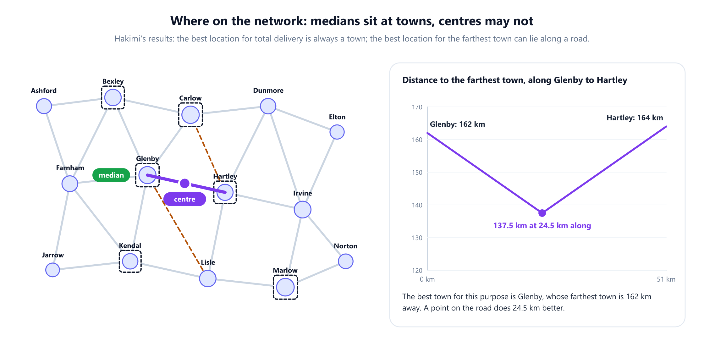
If the only question is how far the farthest town is, the best town in this region is again Glenby, whose farthest town is 162 km away. But standing on the road from Glenby to Hartley, 24.5 km out of Glenby, the farthest town is only 137.5 km away, 24.5 km better than any town. Moving along that road brings the far western and eastern towns closer at the same rate that it pushes the others away, and the best point is where the two sides balance.
The practical lesson is to match the candidate list to the objective. For cost-driven distribution networks, candidate sites at towns or road junctions lose nothing, by Hakimi's median theorem. For coverage-driven decisions, such as promising every customer a delivery within a time limit or placing ambulance stations, the best location can fall between junctions, and the candidate list should include points along roads.
8. How many warehouses?
The number of warehouses is a decision in its own right, and the exact model answers it by finding the cheapest network for each count.
| Warehouses | Cheapest sites | Total per year |
|---|---|---|
| 1 | None has enough capacity | Not feasible |
| 2 | Glenby, Marlow | $857,840 |
| 3 | Carlow, Glenby, Marlow | $850,240 |
| 4 | Bexley, Hartley, Kendal, Marlow | $881,840 |
| 5 | Bexley, Carlow, Glenby, Kendal, Marlow | $920,320 |
| 6 | All six | $980,240 |
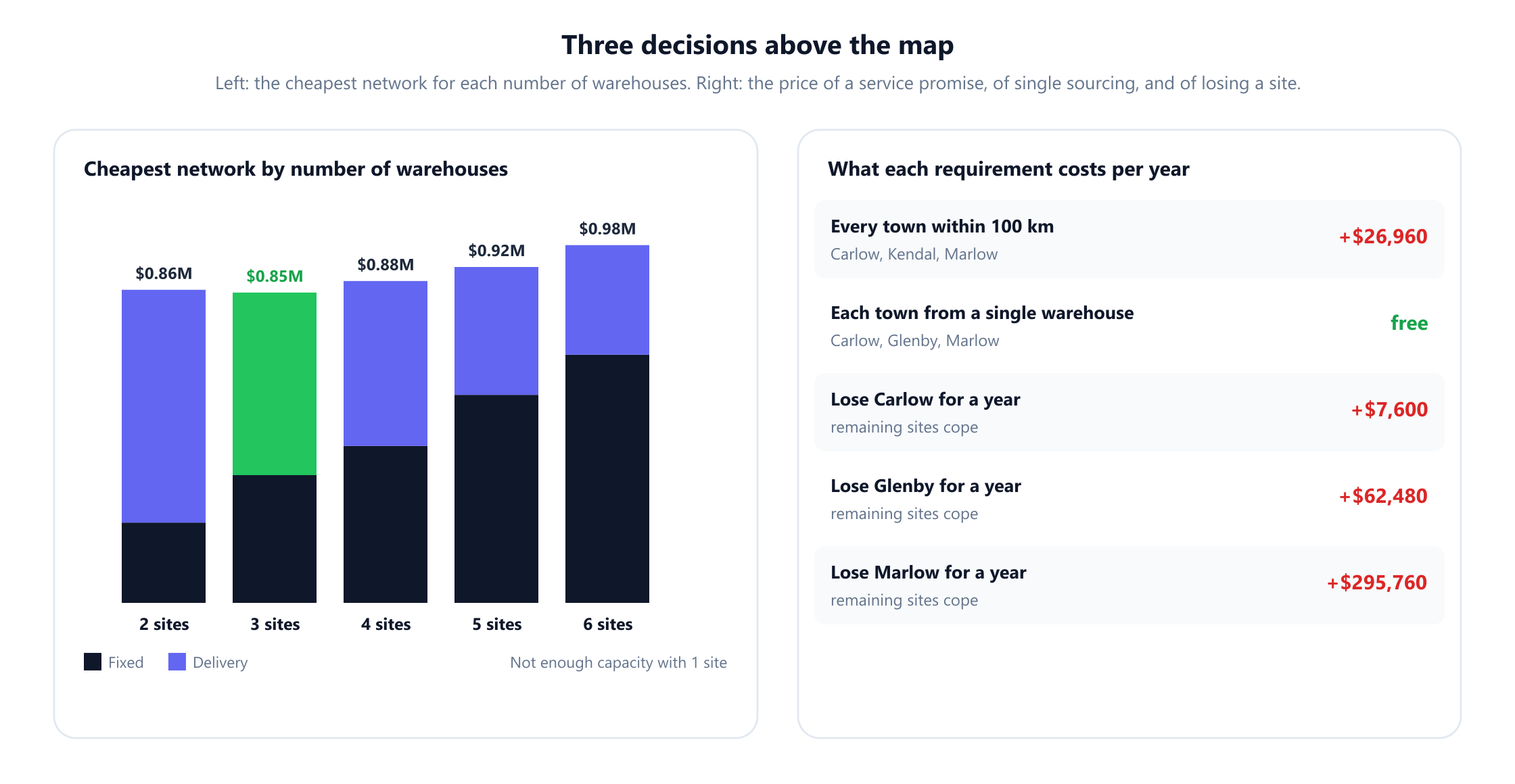
Three warehouses win, but only just. The best two-site network, Glenby and Marlow, costs $7,600 a year more, less than 1% of the total. Beyond three the curve rises steeply, because each extra site adds more than $100,000 of fixed cost and saves far less in delivery.
A flat curve near the optimum is common, and it changes what the decision is really about. When two options are within 1% on cost, the model has not failed to decide; it has shown that cost is no longer the deciding factor, and that service, growth and resilience should be. Sections 9 and 11 show that on those measures the two options are very different.
9. Pricing a service promise
Suppose the sales team wants to promise every customer next-morning delivery, which the operation can guarantee only if every town is within 100 km of the warehouse that serves it.
The optimal network breaks that promise in exactly one place: Jarrow, a small town of 5,000 tonnes a year, is 113 km from its nearest open warehouse at Glenby. Re-solving with the promise as a constraint gives a different network, Carlow, Kendal and Marlow, costing $877,200 a year. The promise costs $26,960 a year, about 3.2% of the network, almost all of it to reach one small town.
The model also shows the limit of what can be promised at all. With these six candidate sites, no combination can bring every town closer than 99 km to an open warehouse, so a 90 km promise is impossible without a new site, whatever it costs.
Coverage constraints like this have their own family of models. The location set covering problem of Toregas, Swain, ReVelle and Bergman (1971) finds the fewest facilities that cover every customer within a distance, and the maximal covering location problem of Church and ReVelle (1974) covers as much demand as possible with a fixed number of facilities. Both were developed for emergency services, and both are how a service promise turns into a location decision.
10. Single sourcing
The transportation model allows a town's volume to be split between two warehouses if that is cheaper, but many companies insist that each customer is served by exactly one warehouse, which keeps ordering, invoicing and delivery windows simple. That requirement turns the flow problem into an assignment problem with capacities, which is harder to solve.
On this region the rule is free: the optimal network already serves every town from a single warehouse, so imposing it changes nothing. That is not luck so much as slack: each open warehouse runs well below capacity, so the model never needs to split a town. When warehouses run close to full, single sourcing can force a large customer onto a more distant site and cost real money, which is exactly when it should be priced before being made policy.
11. Losing a warehouse
A network is chosen for normal operation, but warehouses flood, burn, strike or lose their lease. The same model prices each failure by removing one open site and re-optimising deliveries from the other two.
| Site lost for a year | Network left | Total per year | Extra cost |
|---|---|---|---|
| Carlow | Glenby, Marlow | $857,840 | +$7,600 |
| Glenby | Carlow, Marlow | $912,720 | +$62,480 |
| Marlow | Carlow, Glenby | $1,146,000 | +$295,760 |
The spread is the lesson. Losing Carlow barely matters, because the remaining two sites are the second-best network anyway. Losing Marlow, one of the two cheapest sites to run, costs $295,760, more than a third of the network's annual cost, because Marlow is the only open site in the south-east and everything it served would be driven from Carlow and Glenby.
The fixed cost of a site says nothing about how critical it is. Reliability models, such as Snyder and Daskin's 2005 expected failure cost formulation, build these failure scenarios into the location decision itself, and they often recommend a network that costs slightly more in normal operation and far less when something goes wrong.
12. What is easy, what is hard
| Question | Graph or model view | Difficulty |
|---|---|---|
| Road distance between every town and site | All-pairs shortest paths | Polynomial |
| Cheapest deliveries from a fixed set of open sites | Transportation problem, minimum cost flow | Polynomial |
| Best single location for total delivery | 1-median, which lies at a vertex | Polynomial: check every vertex |
| Best single location for the farthest customer | Absolute 1-centre | Polynomial: check every edge |
| Best p locations on a tree network | p-median or p-centre on a tree | Polynomial |
| Best p locations on a general network | p-median, p-centre | NP-hard (Kariv and Hakimi, 1979) |
| Which sites to open with fixed costs and capacities | Capacitated facility location | NP-hard |
The pattern is the same as in supply chain optimization: moving goods through a fixed network is easy, and deciding which discrete facilities should exist is hard. The saving grace is that for any fixed choice of sites the rest is a flow problem, which is why exact methods that branch on the site decisions and solve flows at each step work well in practice.
13. What the model leaves out
- Inbound freight. Goods arrive at warehouses from plants, ports or suppliers, and that cost also depends on location. A full network design model includes both legs.
- Inventory. Fewer warehouses usually mean less safety stock, because variability pools. Maister's 1976 square root law estimates the effect, and it can favour fewer, larger sites than delivery cost alone suggests.
- Growth and time. A network built for this year's volume will run for a decade. Multi-period models open sites in stages as demand grows, and scenarios test the choice against several futures.
- Uncertain demand. Volumes by town are forecasts. Snyder's 2006 review covers stochastic and robust location models that hedge against them.
- Economies of scale. Real fixed costs and handling costs are not linear in size, and a site can often be built in several capacity options.
- Site realities. Labour availability, planning permission, access to motorways and local taxes all rule sites in or out before any optimisation runs.
None of these changes the core picture: a road graph, candidate sites, a cost for opening each, and a flow problem for serving customers. They change the data and add constraints. Once the warehouses exist, the daily question becomes routing the vehicles that leave them, covered in delivery route optimization.
14. Running a location study
Start from shipment data, not a map. A year of deliveries by customer location, with weights or volumes, gives the demand. Road distances or drive times come from a routing engine, and delivery rates from carrier contracts or the fleet's own costs.
Use the centre of gravity for screening only. It is a reasonable way to find the general area worth looking at, and a poor way to choose a building. Generate a list of real candidate sites, then evaluate them on road distances with an optimisation model.
Price the current network first. Model today's warehouses with the same data and costs. That baseline shows how much is at stake and whether the model reproduces reality before anyone trusts its recommendations.
Use a solver and run scenarios. Mixed integer programming solvers such as HiGHS, Gurobi and CPLEX, used through modelling tools such as Pyomo or PuLP, solve realistic location models, and commercial network design tools package the same methods with data preparation. The most valuable output is rarely a single answer: it is a table of scenarios showing how the best network changes with volume growth, fuel prices, service promises and the loss of a site.
15. Mistakes that quietly cost money
- Measuring straight lines. Here roads were 28% longer on average and up to 1.91 times longer. The straight-line plan cost $114,880 a year more.
- Choosing sites one at a time. ADD locked in Hartley in its first step and never let it go, costing $21,600 a year.
- Minimising the cost of buildings. Both worse plans spent less on fixed cost and far more on delivery.
- Treating the number of warehouses as fixed. Two and three warehouses were within 1% on cost and very different on service and risk. Solve for each count.
- Making a service promise without pricing it. A 100 km promise cost $26,960 a year, mostly for one small town, and a 90 km promise was impossible with these sites.
- Judging criticality by site cost. Losing Marlow, one of the cheapest sites, cost $295,760 a year.
- Using a median model for a coverage question. For the farthest customer the best point was on a road, 24.5 km better than any town.
- Designing for one year. A warehouse outlives its first forecast. Test the network against growth and alternative futures.
16. Frequently asked questions
What is the facility location problem?
+
It is the problem of choosing where to open facilities, such as warehouses, plants or service centres, and which customers each one serves, so that the total of fixed facility costs and delivery costs is as low as possible while capacities and service requirements are respected. On a road network the customers and candidate sites are vertices of a graph, and the delivery cost depends on shortest path distances between them.
How do I decide where to put a new warehouse?
+
Collect a year of shipment data by customer location, draw up a list of real candidate sites with their fixed costs and capacities, compute road distances from each site to each customer, and solve a facility location model that chooses sites and assignments together. Price your current network the same way as a baseline, then test the recommended network against growth, service promises and the loss of a site before committing.
Is the centre of gravity method good enough?
+
It is useful for finding the general area to look in and unreliable for choosing a site. It measures straight-line distance, ignores fixed costs and capacities, and produces points that must then be snapped to real sites. In this article's example, snapping three straight-line centres to the nearest candidate sites gave a network costing $114,880 a year more than the best network found on road distances.
How many warehouses does a business need?
+
Enough that adding another would cost more in fixed cost than it saves in delivery, which a location model finds by solving for each possible count. The cost curve is often flat near the best number: in this article's example, two and three warehouses were within $7,600 a year of each other, so the choice between them should be made on service promises, growth and resilience rather than cost alone.
What is the difference between the p-median and p-centre problems?
+
The p-median problem places p facilities to minimise the total demand-weighted distance to customers, which models delivery cost. The p-centre problem places them to minimise the distance to the farthest customer, which models a service guarantee. Hakimi showed that an optimal median can always be found at vertices of the network, while an optimal centre may lie partway along an edge. On general networks both problems are NP-hard.
Why is facility location hard to solve?
+
Because the decisions about which sites to open are yes-or-no choices, and their number of combinations doubles with every candidate site: six sites give 63 combinations, but thirty give more than a billion. Capacitated facility location and the p-median problem on general networks are NP-hard. For any fixed set of sites, though, serving customers is a polynomial flow problem, which is why branch and bound methods solve real instances well.
What software is used for warehouse location and network design?
+
Mixed integer programming solvers such as HiGHS, Gurobi and CPLEX solve facility location models directly, usually through a modelling layer such as Pyomo, PuLP or JuMP, with road distances from a routing engine. Commercial supply chain network design tools package the same optimisation with data preparation and scenario management. Spreadsheet centre of gravity tools are common but, as the example shows, should only be used for screening.
17. References
The foundational papers, surveys and books behind the methods in this article, in chronological order.
- Weber, A. (1909). Über den Standort der Industrien. Tübingen: J. C. B. Mohr.
- Weiszfeld, E. (1937). “Sur le point pour lequel la somme des distances de n points donnés est minimum.” Tôhoku Mathematical Journal, 43, 355–386.
- Hitchcock, F. L. (1941). “The distribution of a product from several sources to numerous localities.” Journal of Mathematics and Physics, 20(1–4), 224–230.
- Kuehn, A. A. and Hamburger, M. J. (1963). “A heuristic program for locating warehouses.” Management Science, 9(4), 643–666.
- Cooper, L. (1964). “Heuristic methods for location-allocation problems.” SIAM Review, 6(1), 37–53.
- Hakimi, S. L. (1964). “Optimum locations of switching centers and the absolute centers and medians of a graph.” Operations Research, 12(3), 450–459.
- Balinski, M. L. (1965). “Integer programming: methods, uses, computation.” Management Science, 12(3), 253–313.
- Hakimi, S. L. (1965). “Optimum distribution of switching centers in a communication network and some related graph theoretic problems.” Operations Research, 13(3), 462–475.
- Feldman, E., Lehrer, F. A. and Ray, T. L. (1966). “Warehouse location under continuous economies of scale.” Management Science, 12(9), 670–684.
- Teitz, M. B. and Bart, P. (1968). “Heuristic methods for estimating the generalized vertex median of a weighted graph.” Operations Research, 16(5), 955–961.
- Toregas, C., Swain, R., ReVelle, C. and Bergman, L. (1971). “The location of emergency service facilities.” Operations Research, 19(6), 1363–1373.
- Church, R. and ReVelle, C. (1974). “The maximal covering location problem.” Papers of the Regional Science Association, 32(1), 101–118.
- Maister, D. H. (1976). “Centralisation of inventories and the ‘square root law’.” International Journal of Physical Distribution, 6(3), 124–134.
- Erlenkotter, D. (1978). “A dual-based procedure for uncapacitated facility location.” Operations Research, 26(6), 992–1009.
- Kariv, O. and Hakimi, S. L. (1979). “An algorithmic approach to network location problems. I: The p-centers” and “II: The p-medians.” SIAM Journal on Applied Mathematics, 37(3), 513–538 and 539–560.
- Owen, S. H. and Daskin, M. S. (1998). “Strategic facility location: a review.” European Journal of Operational Research, 111(3), 423–447.
- Snyder, L. V. and Daskin, M. S. (2005). “Reliability models for facility location: the expected failure cost case.” Transportation Science, 39(3), 400–416.
- Snyder, L. V. (2006). “Facility location under uncertainty: a review.” IIE Transactions, 38(7), 547–564.
- Melo, M. T., Nickel, S. and Saldanha-da-Gama, F. (2009). “Facility location and supply chain management: a review.” European Journal of Operational Research, 196(2), 401–412.
- Daskin, M. S. (2013). Network and Discrete Location: Models, Algorithms, and Applications, 2nd edition. Hoboken: Wiley.