
Table of Contents
- 1. Why a supply chain is a graph
- 2. The anatomy: vertices, arcs and the numbers on them
- 3. The network used throughout this article
- 4. Lead time: shortest paths
- 5. Capacity: maximum flow and the cut that limits you
- 6. Cost: the transportation problem and minimum cost flow
- 7. Which warehouses should exist at all?
- 8. Designing the physical network: spanning trees
- 9. The last mile: routing the vehicles
- 10. Inside the factory: materials and schedules
- 11. Resilience: what breaks, and how badly
- 12. Two modelling tricks worth knowing
- 13. What is easy, what is hard
- 14. From model to practice
- 15. Modelling mistakes that produce confident wrong answers
- 16. Frequently asked questions
- 17. References
1. Why a supply chain is a graph
A supply chain is a set of places and a set of movements between them. Suppliers ship to plants, plants ship to warehouses, warehouses ship to stores, and something is true or false about every possible movement: it exists or it does not, it costs this much per unit, it takes this many days, it can carry at most this much per week.
That description is already a graph. The places are vertices, the movements are directed arcs, and the commercial facts are numbers attached to the arcs. Nothing has been simplified away yet, and the moment the model exists, a century of algorithms becomes available: shortest path answers "how fast can this reach that", maximum flow answers "how much can we actually deliver", minimum cost flow answers "what is the cheapest plan", and connectivity answers "what happens when this burns down".
This is not a metaphor invented for teaching. The mathematics of supply chains is network optimisation. Hitchcock posed the transportation problem in 1941 and Koopmans reached it independently in work presented in 1947 and published in 1949; Dantzig solved it with the simplex method in 1951; Ford and Fulkerson published the maximum flow algorithm in 1956 and the book Flows in Networks in 1962, and their examples were railway capacity and shipment planning rather than abstract graphs. The field that formalised all of it is operations research, and its central objects are graphs.
What this article does is take one small network, four echelons wide, and answer every standard supply chain question on it. Every number quoted below was computed by solving the model, not estimated: the plans, the bottlenecks, the shortfalls after a failure, and the cost of each alternative. If you are new to the underlying vocabulary, the introduction to graph theory covers the definitions this article assumes.
2. The anatomy: vertices, arcs and the numbers on them
Modelling is the act of deciding what to keep. Three decisions carry most of the weight.
What is a vertex? Usually a physical location: a supplier site, a plant, a distribution centre, a customer region. Sometimes it is finer, such as a production line or a dock door, and sometimes coarser, such as a whole country in a strategic study. The rule is that a vertex is anything you might want to open, close, capacitate or lose, because those are the questions the model will be asked.
What is an arc? A lane: an origin, a destination, and usually a mode. The same two facilities connected by road and by air are two arcs, not one, because they have different costs, times and capacities. Arcs are directed, since shipping east is not the same as shipping west; the distinction and its consequences are covered in directed versus undirected graphs.
What goes on the arc? At least three numbers, and they answer different questions, so it matters which one you attach:
- Capacity, in units per period. This limits what is possible and is the input to maximum flow.
- Cost, per unit shipped. This decides what is cheapest and is the input to minimum cost flow.
- Transit time, in days. This decides what is fast and is the input to shortest path.
Beginners often collapse these into one "weight" and then wonder why the answer looks wrong. They are genuinely different objectives, and the cheapest route is frequently not the fastest one, as section 4 shows on this very network. The guide to weighted versus unweighted graphs makes the same point in the abstract.
Two more attributes live on vertices rather than arcs: supply at the sources, demand at the sinks, and sometimes a fixed cost for a facility to exist at all, which is what turns a flow problem into a location problem in section 7.
3. The network used throughout this article
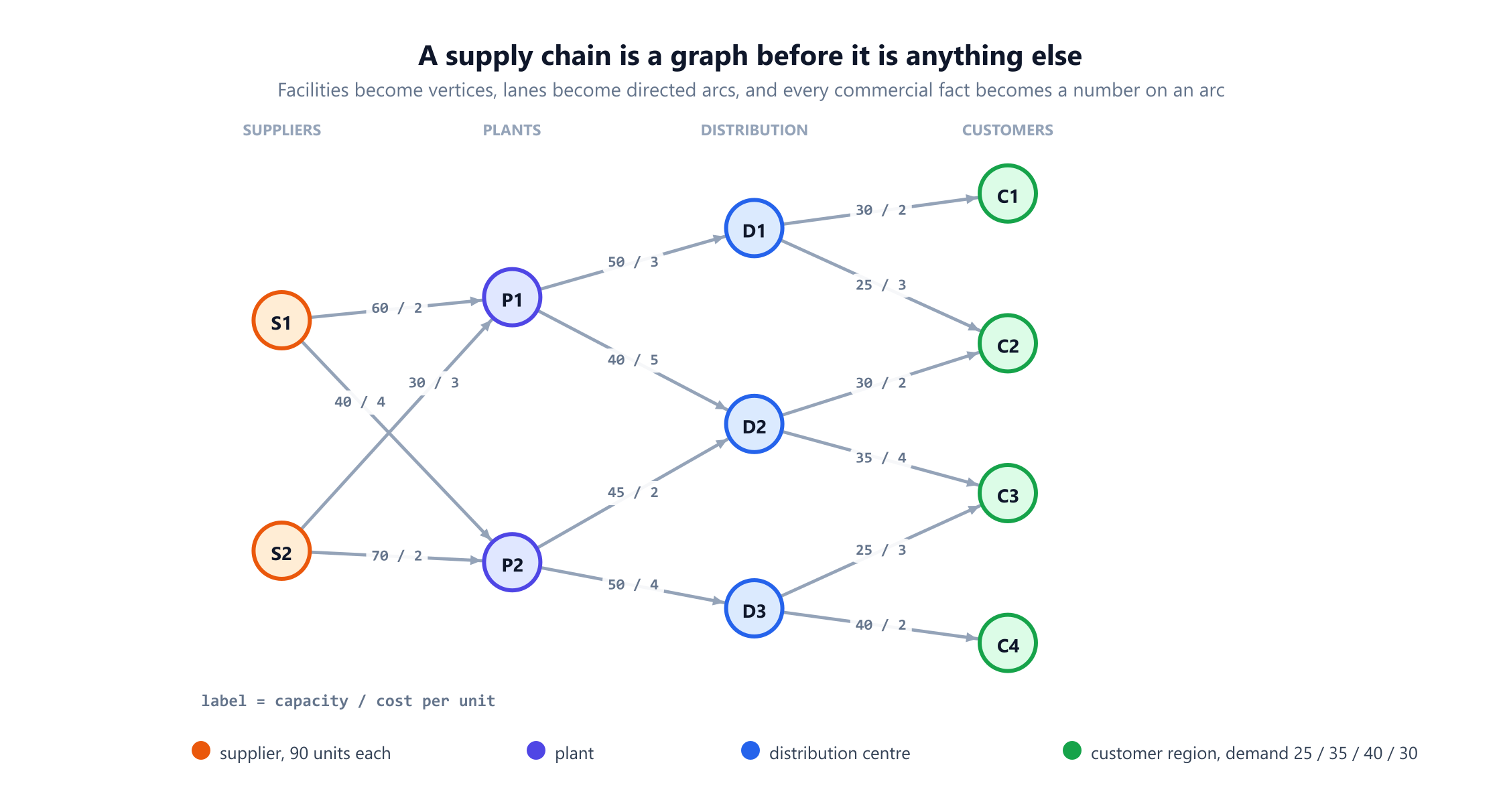
The running example is deliberately small enough to check by hand and rich enough to break in interesting ways. Two suppliers feed two plants, the plants feed three distribution centres, and the centres serve four customer regions.
| Echelon | Nodes | Numbers |
|---|---|---|
| Suppliers | S1, S2 | 90 units per week available at each |
| Plants | P1, P2 | Convert supply into finished goods |
| Distribution centres | D1, D2, D3 | Capacities 55, 75 and 65 units |
| Customers | C1, C2, C3, C4 | Demand 25, 35, 40 and 30, totalling 130 |
Each of the fourteen lanes carries a capacity, a cost per unit and a transit time, as drawn in the figure above. Total supply is 180 against demand of 130, so in the base case there is slack; section 5 removes it.
One structural detail matters before any algorithm runs. The network is a directed acyclic graph: material only ever moves left to right, from supply towards demand. Real chains have returns, rework loops and transfers between warehouses, all of which create cycles, and the algorithms below still work. But the acyclic case is the one where the intuition is cleanest, and it is where most tactical planning models actually live.
A second detail is that this is a single product, single period model. That assumption is doing a lot of work, and section 12 shows the standard graph construction that removes it.
4. Lead time: shortest paths
The first question anyone asks of a network is how quickly it can respond. With transit times on the arcs, that is exactly the shortest path problem, and Dijkstra's algorithm answers it for every destination at once in O(m + n log n).
Solving it from each supplier gives the service picture:
| From | C1 | C2 | C3 | C4 |
|---|---|---|---|---|
| S1 | 6 days S1-P1-D1-C1 | 7 days S1-P1-D1-C2 | 9 days S1-P2-D3-C3 | 8 days S1-P2-D3-C4 |
| S2 | 7 days S2-P1-D1-C1 | 6 days S2-P2-D2-C2 | 6 days S2-P2-D3-C3 | 5 days S2-P2-D3-C4 |
Three things fall out of this table that a spreadsheet would not have told you. The worst service in the network is 9 days, from S1 to C3, and it is the number a service level agreement has to be written against. The two suppliers are not interchangeable: S1 is faster to C1, S2 is faster to everything else, which is an argument for dual sourcing by region rather than by volume. And the fastest route to C3 from S1 goes through P2, not through the geographically obvious P1, because the P1 branch is slower at every step.
Now compare with cost. The cheapest lane out of S1 is S1 → P1 at 2 per unit, and the fastest route to C3 avoids it entirely. Minimising days and minimising money are different optimisations over the same graph, and any planning tool that offers a single "best route" is quietly choosing one of them for you. The full decision tree of which algorithm applies to which variant is in shortest path algorithms.
Two practical extensions are worth knowing. Adding a fixed handling time at each facility is done by putting the delay on the node, which section 12 turns into an arc. And when the question is "what is the fastest route that also costs less than X", you have a constrained shortest path problem, which is NP-hard in general and usually solved with Lagrangian relaxation or a labelling algorithm rather than plain Dijkstra.
5. Capacity: maximum flow and the cut that limits you
The second question is how much the network can actually move. Add an artificial source feeding both suppliers with their available volume, and an artificial sink drawing each customer's demand, and the answer is a maximum flow computation.
In the base case the answer is undramatic: all 130 units get through. What makes it interesting is where the binding constraint sits. Solving the flow problem also produces the minimum cut, and here the cut consists of the customer arcs themselves. In plain language: nothing inside the network is limiting anything, and the only reason more units do not flow is that nobody has ordered them. That is the healthy case, and it is worth confirming before anyone is asked to approve capital expenditure.
Now raise every demand by 40%, a modest peak season. Demand becomes 182 units, and the network delivers 164.
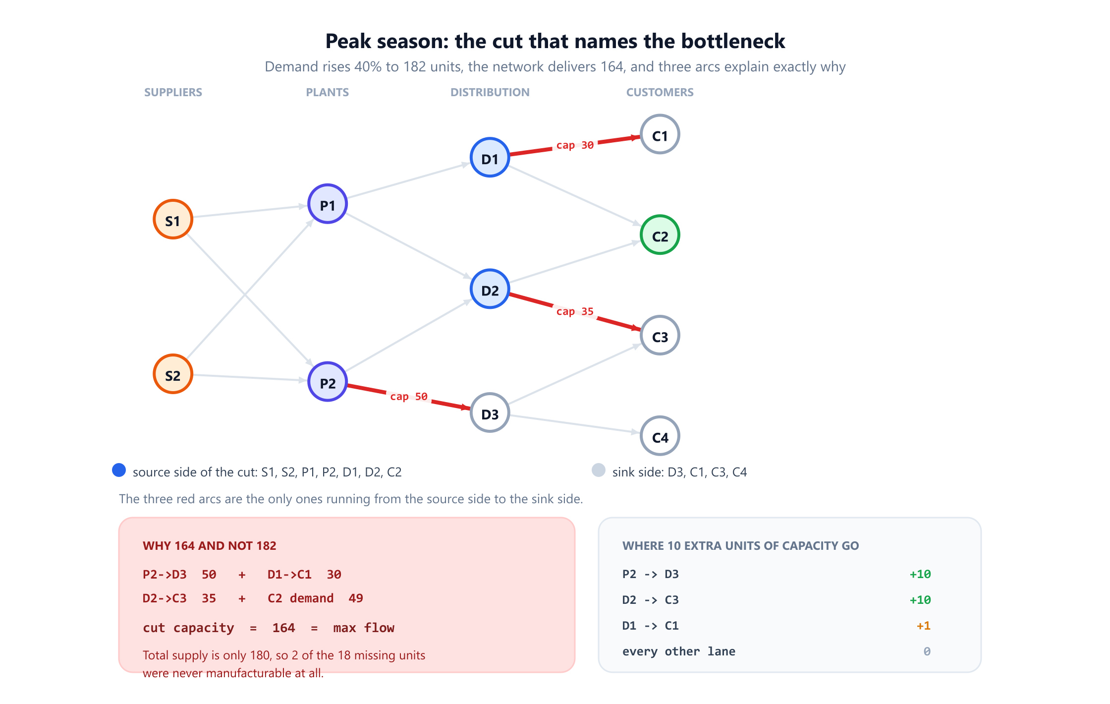
The 18 missing units decompose precisely. Total supply is 180, so 2 units were never manufacturable regardless of the network. The remaining 16 are lost to structure, and the minimum cut names the structure exactly: P2 → D3 at capacity 50, D1 → C1 at 30, D2 → C3 at 35, plus the 49 units of C2 demand that sits on the source side. Those add to 164, which the max-flow min-cut theorem guarantees equals the maximum flow, and the arithmetic confirms it.
This is the single most useful thing graph theory does for a supply chain, so it is worth stating plainly. The minimum cut is the investment list. Capacity added anywhere else changes nothing at all. Testing that claim on this network gives a result that no amount of intuition would produce:
- 10 extra units on
P2 → D3: throughput rises from 164 to 174. - 10 extra units on
D2 → C3: also 174. - 10 extra units on
D1 → C1: throughput rises to 165, and no further. One unit, not ten. - 10 extra units on any of the other eleven lanes: no change whatsoever.
The D1 → C1 case is the instructive one. It is genuinely on the minimum cut, so the first unit of extra capacity does help, but after that a different constraint binds and the investment stops paying. A cut tells you where the wall is today; it does not promise the wall stays in the same place once you move it. In practice this is why capacity planning is done as a sequence of re-solves rather than a single ranking.
6. Cost: the transportation problem and minimum cost flow
Feasibility is not a plan. The operational question is which of the many feasible plans is cheapest, and that is the minimum cost flow problem: satisfy every demand, respect every capacity, minimise the sum of flow times cost over all arcs.
Its ancestor is the transportation problem, posed by Hitchcock in 1941 and independently by Koopmans, and solved efficiently by Dantzig in 1951 with a specialised simplex method. The modern general form is solved by the network simplex algorithm or by successive shortest paths, and Ahuja, Magnanti and Orlin's Network Flows remains the standard treatment.
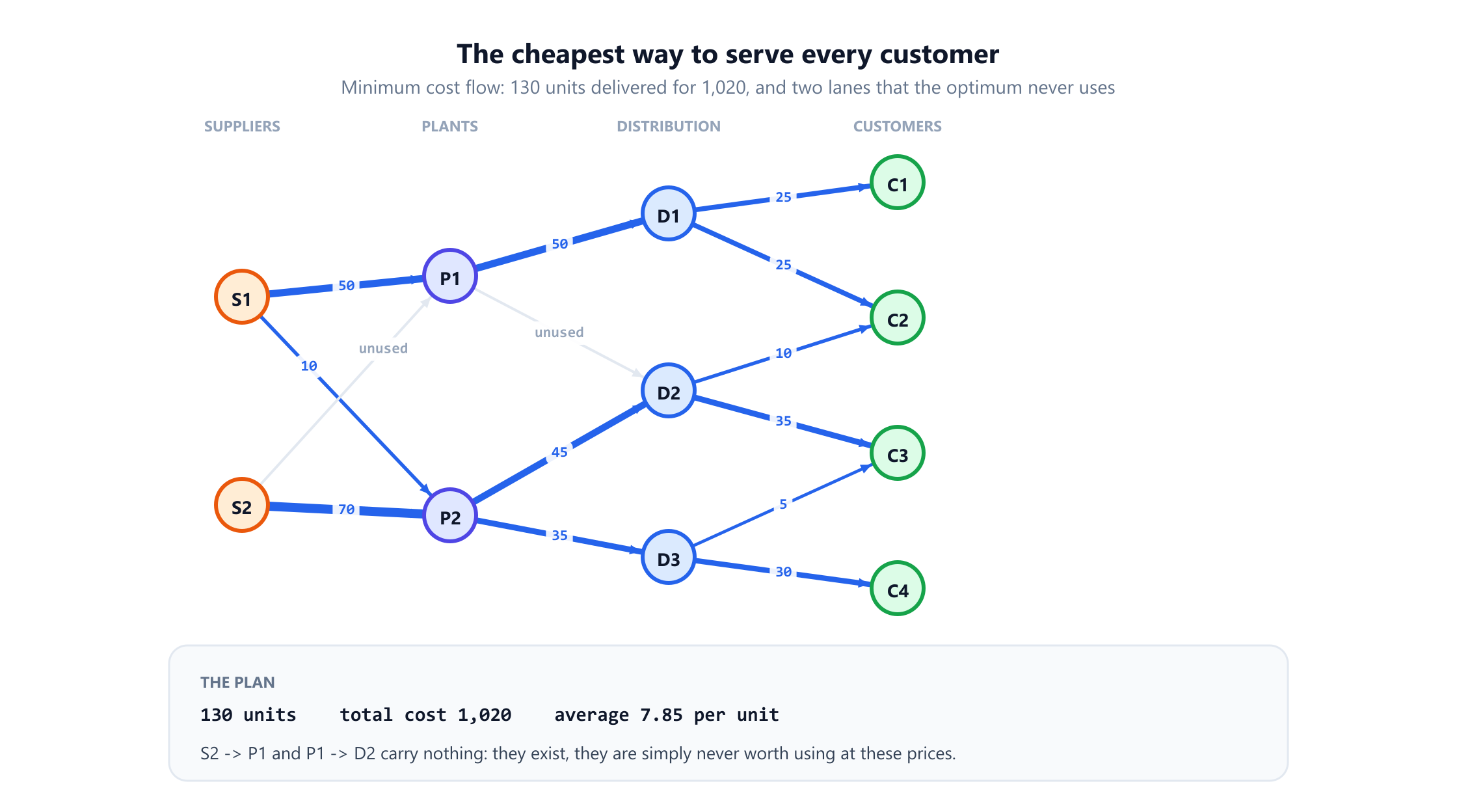
Solved on the running network, the cheapest way to deliver all 130 units costs 1,020, an average of 7.85 per unit:
Three features of the solution are worth reading carefully, because they are the features that surprise people.
Two lanes carry nothing. S2 → P1 and P1 → D2 are perfectly usable and are never worth using at these prices. A network diagram cannot tell you this; only the optimisation can. It is also the answer to "why do we pay to maintain that lane", which is a question worth asking annually.
Demand gets split. C2 is served 25 units from D1 and 10 from D2, and C3 is served 35 from D2 and 5 from D3. Single sourcing each customer from its nearest centre is a rule of thumb, not an optimum, and here it would cost more. Real models often add a constraint forbidding splits, and the price of that constraint should be measured rather than assumed.
The answer came out in whole units. That is not luck. The constraint matrix of a network flow problem is totally unimodular, so when supplies and demands are integers, the linear program has an integer optimal solution automatically. This is why flow problems are solved as linear programs and still give shippable answers, and it is exactly what fails the moment you add a binary "open or closed" decision, which is the subject of the next section.
7. Which warehouses should exist at all?
Everything so far took the network as given. The strategic question is which facilities should exist, and it changes the mathematics completely: opening a site costs a fixed amount whether it ships one unit or a thousand, and a fixed cost cannot be expressed as a cost per unit on an arc.
Give the three distribution centres a weekly fixed cost of 250, 300 and 200, capacities of 55, 75 and 65 units, and a cost per unit for serving each customer region. Then the question is which subset to open, and for each candidate subset the serving cost is itself a transportation problem. With three sites there are seven subsets and we can simply solve all of them.
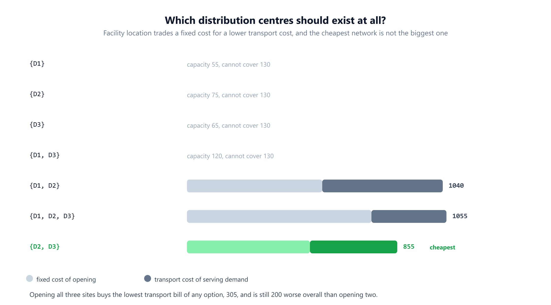
The winner is {D2, D3} at 855: 500 of fixed cost and 355 of transport. The result that matters pedagogically is the last row. Opening all three centres produces the lowest transport cost of any configuration, 305, because every customer can then be served from its cheapest source. It is still 200 worse in total, because the third site's fixed cost of 250 buys only 50 of transport savings. Optimising the flow inside a network you have already over-built is a good way to be efficiently wrong.
This is the capacitated facility location problem, and unlike everything in sections 4 to 6 it is NP-hard. With three candidate sites, brute force over eight subsets is instant. With three hundred, it is not, and the field solves it with mixed integer programming: Balinski gave the standard formulation in 1965, Geoffrion and Graves solved a real multi-commodity distribution design with Benders decomposition in 1974, and modern solvers handle industrial instances routinely. The structure that makes it tractable in practice is exactly the one visible here: for any fixed set of open sites, the remaining problem is a network flow that solves in polynomial time. A fuller worked example, with road distances, the classic siting heuristics and the price of a service promise, is in facility location: where to put your next warehouse.
8. Designing the physical network: spanning trees
A different design question is not "where should facilities be" but "which connections should we build". Laying a private line, contracting a dedicated shuttle, or building a rail spur has a cost per link, and the requirement is that every facility can reach every other.
That is the minimum spanning tree problem, solved by Kruskal's algorithm in O(m log n). On six facilities, two plants, three centres and a shared cross-dock hub, with eleven possible links priced between 3 and 10, the cheapest connected design costs 21 and uses five links: P2-H at 3, P1-D1 at 4, D2-H at 4, P2-D3 at 5 and D1-H at 5.
Five links for six facilities is not a coincidence. A tree on n vertices always has exactly n - 1 edges, and that is the defining trade-off of the whole approach: a spanning tree is the cheapest way to connect everything, and it is also the most fragile way. Every one of those five links is a bridge, meaning its loss disconnects the network, and three of the six facilities are cut vertices. Section 11 puts numbers on what that costs.
The practical lesson is that minimum spanning tree is the right algorithm for the wrong objective in most supply chain settings. What you usually want is the cheapest network that survives the loss of any single link, which is two-edge-connected network design, and that problem is NP-hard. The MST is still worth computing, because it is a lower bound: no connected design can cost less, so it tells you the price of the redundancy you are about to buy.
9. The last mile: routing the vehicles
Everything above moves units between facilities. The final leg moves them to doors, and it is where a large share of distribution cost is incurred and where the mathematics gets hard.
Give one vehicle a set of stops and ask for the shortest tour that visits each exactly once and returns to the depot, and you have the travelling salesperson problem. Give a fleet with capacities and ask which vehicle serves which stops, and you have the vehicle routing problem, introduced by Dantzig and Ramser in 1959 under the name "the truck dispatching problem" and generalised ever since into windows, mixed fleets, pickup and delivery, and driver hours.
The difference from sections 4 to 6 is a difference in kind, not in degree. Shortest path, max flow and min cost flow are all polynomial: a modern solver handles a continental road network in under a second. TSP and VRP are NP-hard, and the number of possible tours through n stops is (n-1)!/2, which passes 60 quadrillion at just 20 stops. That is why practice runs on heuristics: the Clarke and Wright savings algorithm from 1964 is still a standard construction method, local search such as 2-opt and Or-opt improves the result, and metaheuristics such as large neighbourhood search drive commercial engines. Exact methods have improved enormously too, and instances with hundreds of customers are now solved to proven optimality, but the daily dispatch problem is solved by heuristics because it has to be answered in minutes.
The modelling point worth carrying away: the routing layer sits on top of the flow layer. The flow model decides that D3 ships 30 units to region C4; the routing model decides the sequence of doors within C4 and which truck does it. Optimising them jointly is possible and is what integrated planning systems attempt, but the two-stage split is standard because each stage is hard for a different reason. For the routing layer worked end to end and priced in fleet costs, see delivery route optimization.
10. Inside the factory: materials and schedules
Zoom into a single plant and the graphs do not stop. Two of them run the factory, and both are directed acyclic graphs answered by one pass in topological order.
The first is the bill of materials. A product is made of components, each of which is made of components, and the arcs carry quantities. Exploding a customer order into raw material requirements means walking that graph from the top down, multiplying as you go. This is what material requirements planning does, formalised by Orlicky in 1975 and still the core loop of every ERP system.
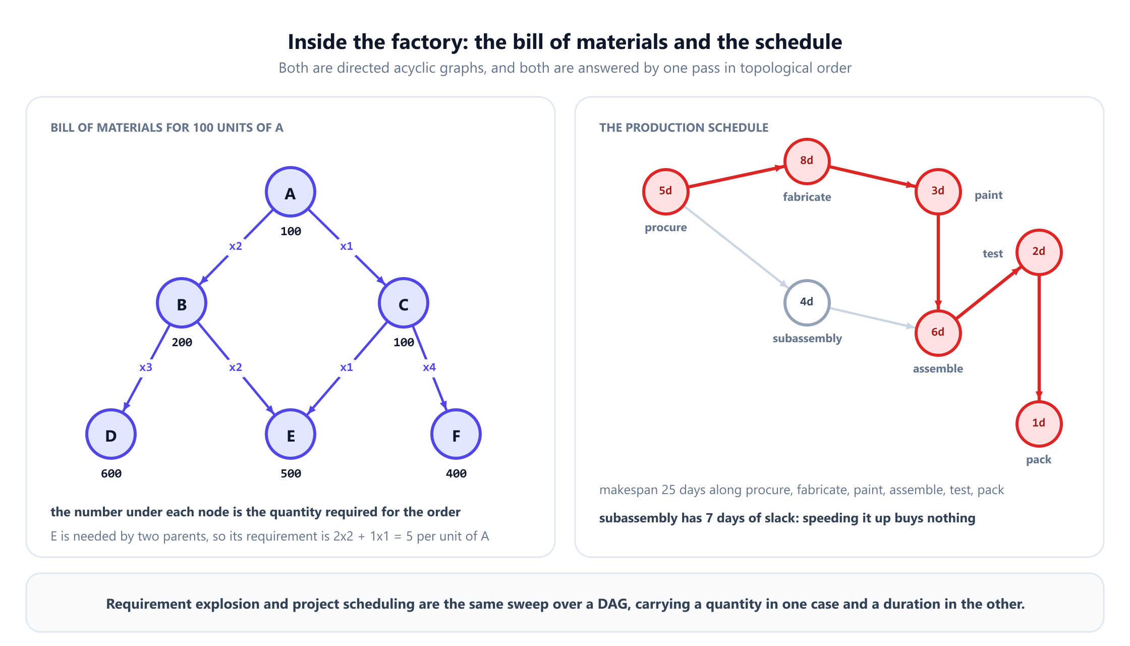
For an order of 100 units of product A, the explosion gives 200 of B, 100 of C, 600 of D, 500 of E and 400 of F. Component E is the one worth pausing on: it appears under two different parents, so its requirement is 2 × 2 through B plus 1 × 1 through C, which is 5 per unit of A. Adding up the branches independently, which is what a naive spreadsheet does, double counts or undercounts precisely these shared components. Processing the items in topological order guarantees every parent is final before a child is read, which is why the sweep is correct in one pass.
The second graph is the schedule. Tasks have durations and precedence constraints, and the project length is the longest path through the resulting DAG. On the seven-task plan in the figure the makespan is 25 days, along procure, fabricate, paint, assemble, test and pack. That chain is the critical path, from Kelley and Walker's 1959 method, and its practical meaning is sharp: any delay on it delays the order one for one, while subassembly carries 7 days of slack and could be delayed a full week without moving the delivery date by an hour.
Note the asymmetry that makes this valuable. Longest path is NP-hard on a general graph and linear on a DAG, so scheduling is cheap precisely because precedence constraints cannot form a cycle. If they do, the plan is infeasible, and the same algorithm detects that too. Sequencing customer orders through the machines themselves, with due dates, colour changes and overtime, is worked through in production scheduling for manufacturers.
11. Resilience: what breaks, and how badly
A cost model tells you what to do when everything works. A resilience model tells you what happens when it does not, and it is the same graph asked a different question: remove a vertex, re-solve the flow, and read the shortfall.
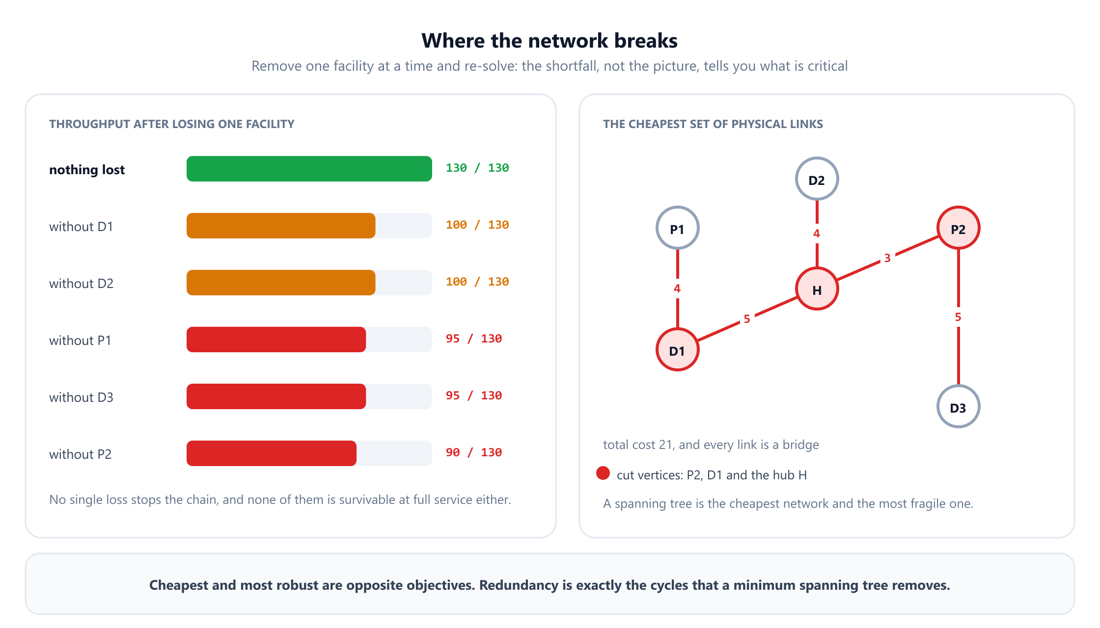
Losing any single facility leaves the network able to deliver between 90 and 100 of the 130 units. The worst case is P2, at 90 units, a 31% shortfall, and that result is worth reading against section 6. The cheapest plan routes 70 units through S2 → P2 and 80 units through P2 in total, because P2 sits on the cheapest lanes. Cost optimisation concentrates flow, and concentrated flow is exactly what fragility looks like. The optimum and the risk are produced by the same property of the network.
Individual lanes matter too, and unequally. The worst single lane is P2 → D3, whose loss costs 35 units; P1 → D1 and D3 → C4 cost 30 each; D2 → C3 costs 20; and S1 → P1, D1 → C2 or D3 → C3 cost only 5. Ranking mitigation spending by lane volume would get this ordering wrong, because volume is what the plan chose to send, not what the network would lose.
The structural view from section 8 says the same thing in a different language. In a minimum spanning tree every link is a bridge and several facilities are cut vertices, so a cost-minimal physical network has, by construction, no redundancy at all. Redundancy is the cycles that the spanning tree removed. Buying resilience means deliberately buying edges that a cost model would reject.
Two research threads are worth naming here. Sheffi's The Resilient Enterprise (2005) made the case that flexibility is a strategic asset rather than waste. And Simchi-Levi and colleagues, working with Ford, formalised the idea that risk should be measured by time to recover and the resulting profit impact rather than by the probability of a disruption, which is unknowable: their 2015 study found that the parts posing the greatest exposure were frequently low-value components from single-source suppliers that no spend-based analysis would ever flag. That is a graph question, and it is the one this section computes.
12. Two modelling tricks worth knowing
Two constructions turn "the model cannot express that" into "the model expresses that fine", and between them they cover most of what beginners hit first.
Node splitting, for capacity on a facility. Flow algorithms put capacity on arcs, but a warehouse has a throughput limit of its own. The fix is to replace the vertex with two: an "in" copy that receives every incoming arc, an "out" copy that sends every outgoing arc, and a single arc between them carrying the facility's capacity.
before:        --> [ D2 ] -->

after:         --> [D2_in] --(capacity 75, cost = handling fee)--> [D2_out] -->
The same trick carries a handling cost or a fixed processing delay, which is how the lead times of section 4 absorb time spent inside a building rather than on a road. It doubles the vertex count and changes nothing else, and every flow algorithm in this article works unmodified afterwards.
Time expansion, for inventory. A single-period model has no memory: whatever is produced must ship immediately. Real chains hold stock, and stock is movement through time rather than space. Build one copy of the network per period and add an arc from each facility in period t to the same facility in period t+1. Flow along that arc is inventory, its cost is the holding cost, and its capacity is the storage limit. How much of that stock to hold, and where, is its own optimisation problem, covered in our guide to inventory optimization and safety stock.
The result is called a time-expanded network, and it is exactly why multi-period production planning is solvable at all: a problem that looks like it needs a new theory turns out to be an ordinary minimum cost flow on a graph T times larger. The same construction handles shelf life, by simply not building the arc that would carry stock past its expiry.
Both tricks share a moral that is worth internalising. When a supply chain feature seems to need a new algorithm, it usually needs a new graph, and the algorithm you already have then applies unchanged.
13. What is easy, what is hard
The most valuable thing a planner can know about their own model is which side of the tractability line it sits on, because that decides whether the answer is an optimum or a good guess.
| Supply chain question | Graph problem | Cost |
|---|---|---|
| Fastest route, service commitments | Shortest path | O(m + n log n) |
| Can we deliver it all? Where is the bottleneck? | Maximum flow, minimum cut | Polynomial |
| Cheapest shipping plan | Minimum cost flow | Polynomial |
| Material requirements | Topological order on a DAG | O(n + m) |
| Project duration, critical path | Longest path on a DAG | O(n + m) |
| Cheapest set of connecting links | Minimum spanning tree | O(m log n) |
| Which facilities to open | Facility location | NP-hard |
| Delivery routes for a fleet | Vehicle routing | NP-hard |
| Cheapest network surviving any single failure | Two-edge-connected design | NP-hard |
| Production batching over time | Lot sizing with setups | NP-hard in general |
The pattern is clean and worth stating: questions about flow are easy, questions about which discrete objects to build are hard. The moment a decision becomes yes or no rather than how much, total unimodularity is lost, the linear program stops handing back integer answers, and you are in mixed integer programming.
Hard does not mean hopeless. Facility location instances with hundreds of candidate sites are solved to proven optimality every day, and vehicle routing heuristics land within a few per cent of the best known solutions on instances far beyond exact methods. What the line changes is the promise: on the top half of the table you can say "this is optimal", and on the bottom half the honest sentence is "this is the best we found, and here is the bound". A fuller treatment of the costs themselves is in graph algorithms and complexity.
14. From model to practice
The gap between a correct model and a useful one is mostly not mathematics. Four things decide whether the work lands.
The data is the project. Lane costs, capacities and transit times live in transport management systems, contracts and spreadsheets, and they disagree with each other. A model built on a lane cost table that is eighteen months old will produce a confident, precise, wrong answer, and the failure will be blamed on the optimisation. Budget most of the effort here.
Choose granularity on purpose. A strategic network study can treat a whole region as one customer vertex; a weekly dispatch model cannot. Aggregating demand is legitimate and aggregating capacity usually is not, because averages hide exactly the peaks that create the bottleneck of section 5.
Use a real solver. For flows, NetworkX and SciPy both ship minimum cost flow, and Google OR-Tools covers flows, routing and scheduling with an interface built for practitioners. For anything with binary decisions, a mixed integer programming solver such as Gurobi, CPLEX or the open-source HiGHS and CBC is the right tool. Writing your own network simplex is a good way to learn and a poor way to ship.
Model the thing that actually varies. A deterministic model answers "what is best if next week is exactly this". Demand is not exactly anything, and the classic failure mode here is not an algorithmic one: Forrester described in 1958 how ordering policies amplify variability upstream, and Lee, Padmanabhan and Whang named it the bullwhip effect in 1997. No amount of optimising a single week's flow addresses it. The standard responses are scenario analysis, stochastic or robust optimisation, and a rolling horizon that re-solves as reality arrives.
One last habit, which the numbers in this article are meant to demonstrate: re-solve rather than reason. The claim that a lane is critical, that a site earns its fixed cost, or that a capacity investment pays back is a claim the model can settle in milliseconds, and intuition about networks is unreliable in exactly the cases that matter. Section 5 found a lane where ten extra units of capacity buys one unit of throughput. Nobody guesses that.
15. Modelling mistakes that produce confident wrong answers
A network model rarely fails loudly. It returns a plan, the plan looks reasonable, and the error is only visible to someone who knows where to look. These are the ones that recur.
- Putting a facility's capacity on one of its arcs. A warehouse that can handle 75 units per week is not the same as a lane that can carry 75, and squeezing the limit onto whichever arc looks busiest quietly permits more or less throughput than reality allows. Split the node, as in section 12.
- Using one number as the arc weight. Cost, time and capacity answer different questions, and a model that carries only one of them will confidently return the cheapest plan when it was asked for the fastest. On this network those two answers genuinely differ.
- Answering a multi-period question with a single-period model. Without inventory arcs, everything produced must ship immediately, so the model will either declare a feasible plan infeasible or invent capacity it does not have. Time-expand the network instead.
- Aggregating capacity along with demand. Averaging four weeks of demand into one is often defensible; averaging capacity is not, because the average hides exactly the peak that creates the bottleneck. The 40% peak in section 5 disappears entirely under monthly averaging.
- Optimising cost with no service constraint. A pure cost objective will happily route everything along the slowest cheap lanes. Lead time has to enter as a constraint or a penalty, or the optimum will be one nobody can operate.
- Ranking risk by volume. The busiest lane is the one the plan chose, which is not the same as the one whose loss hurts most. Re-solve without each candidate and rank by the shortfall, which is what section 11 does and what produces a different ordering.
- Pricing a truckload as a cost per unit. Freight is frequently a step function: the second pallet on a half-empty truck is nearly free, the first pallet on a new truck is not. A linear cost per unit smooths that away and systematically under-values consolidation. Step costs need binary variables, which moves the model into mixed integer programming.
- Forgetting that the arc list is a modelling choice. The optimiser can only choose lanes that exist in the data. A lane nobody entered is a lane that will never appear in the answer, and "the model says we should not use that route" is often just "nobody told the model the route exists".
The common thread is that all eight produce plausible output. The defence is to test the model against a period you already lived through: if it cannot reproduce last quarter's actual flows to within a sensible tolerance, it is not ready to recommend next quarter's.
16. Frequently asked questions
How is graph theory used in supply chain management?
+
Facilities become vertices and shipping lanes become directed arcs, and then the standard questions become standard algorithms: shortest path for lead times and service levels, maximum flow for throughput and bottlenecks, minimum cost flow for the cheapest shipping plan, minimum spanning tree for network design, topological order for bills of materials and production schedules, and facility location and vehicle routing for the strategic and last-mile decisions. Network optimisation is not an analogy for supply chain planning; it is the mathematics the field is built on.
What is the difference between maximum flow and minimum cost flow?
+
Maximum flow asks how much can physically get through and ignores money entirely; it answers "can we serve peak demand, and if not, where is the wall". Minimum cost flow asks for the cheapest way to move a required quantity and ignores anything that is not priced; it answers "given that we can serve demand, what should we actually ship on each lane". In practice you run maximum flow first to check feasibility and find the bottleneck, then minimum cost flow to produce the plan.
Why is the minimum cut so useful in practice?
+
Because it converts a vague statement into a list. The max-flow min-cut theorem says the maximum throughput equals the capacity of the smallest set of arcs whose removal separates supply from demand, so the cut is a precise answer to "which lanes are the constraint". Capacity added anywhere else buys nothing. On the network in this article, ten extra units on either of two named lanes buys ten units of throughput, on a third lane buys one, and on the remaining eleven lanes buys exactly zero.
Is the cheapest network also the best network?
+
Almost never, and graph theory explains why crisply. The cheapest way to connect a set of facilities is a spanning tree, and a spanning tree has no cycles, which means no alternative routes: every link is a bridge whose loss disconnects the network. Redundancy is precisely the set of cycles that a cost-minimising design deletes. The same effect appears in the flow plan, where concentrating volume on the cheapest lanes is what makes a single failure expensive. Cost and resilience are competing objectives and should be priced against each other rather than assumed compatible.
Which supply chain problems are NP-hard?
+
The ones that decide which discrete objects exist. Facility location, vehicle routing, lot sizing with setup costs, and designing a network that survives any single failure are all NP-hard. Everything about flow through a fixed network is polynomial: shortest path, maximum flow, minimum cost flow, spanning trees, topological ordering and critical paths. The dividing line is the moment a decision becomes yes or no rather than how much, because that is when the linear programming relaxation stops returning integer answers by itself.
What software solves these models?
+
For pure network flows, NetworkX and SciPy both ship minimum cost flow solvers, and Google OR-Tools covers flows, routing and scheduling with a practitioner-oriented interface. For anything with binary decisions, such as opening facilities or assigning trucks, use a mixed integer programming solver: Gurobi and CPLEX commercially, HiGHS and CBC in open source, usually through a modelling layer such as Pyomo, PuLP or JuMP. Writing your own network simplex is an excellent way to understand the algorithm and a poor way to ship a planning system.
How do I model inventory held between periods?
+
With a time-expanded network. Make one copy of the whole network for each period and add an arc from each facility in period t to the same facility in period t plus one. Flow along that arc is inventory carried forward, its cost is the holding cost and its capacity is the storage limit. The multi-period problem then becomes an ordinary minimum cost flow on a graph that is T times larger, solvable with exactly the same algorithm. The same construction models shelf life by simply not building the arc that would carry stock past its expiry date.
17. References
The foundational papers and the standard texts, in chronological order.
- Hitchcock, F. L. (1941). “The distribution of a product from several sources to numerous localities.” Journal of Mathematics and Physics, 20(1–4), 224–230.
- Koopmans, T. C. (1949). “Optimum utilization of the transportation system.” Econometrica, 17 (Supplement), 136–146.
- Dantzig, G. B. (1951). “Application of the simplex method to a transportation problem.” In T. C. Koopmans (ed.), Activity Analysis of Production and Allocation, 359–373. New York: Wiley.
- Ford, L. R. and Fulkerson, D. R. (1956). “Maximal flow through a network.” Canadian Journal of Mathematics, 8, 399–404.
- Forrester, J. W. (1958). “Industrial dynamics: a major breakthrough for decision makers.” Harvard Business Review, 36(4), 37–66.
- Dantzig, G. B. and Ramser, J. H. (1959). “The truck dispatching problem.” Management Science, 6(1), 80–91.
- Kelley, J. E. and Walker, M. R. (1959). “Critical-path planning and scheduling.” Proceedings of the Eastern Joint Computer Conference, 160–173.
- Ford, L. R. and Fulkerson, D. R. (1962). Flows in Networks. Princeton: Princeton University Press.
- Clarke, G. and Wright, J. W. (1964). “Scheduling of vehicles from a central depot to a number of delivery points.” Operations Research, 12(4), 568–581.
- Balinski, M. L. (1965). “Integer programming: methods, uses, computation.” Management Science, 12(3), 253–313.
- Geoffrion, A. M. and Graves, G. W. (1974). “Multicommodity distribution system design by Benders decomposition.” Management Science, 20(5), 822–844.
- Orlicky, J. (1975). Material Requirements Planning. New York: McGraw-Hill.
- Ahuja, R. K., Magnanti, T. L. and Orlin, J. B. (1993). Network Flows: Theory, Algorithms, and Applications. Englewood Cliffs: Prentice Hall.
- Lee, H. L., Padmanabhan, V. and Whang, S. (1997). “Information distortion in a supply chain: the bullwhip effect.” Management Science, 43(4), 546–558.
- Sheffi, Y. (2005). The Resilient Enterprise: Overcoming Vulnerability for Competitive Advantage. Cambridge, Massachusetts: MIT Press.
- Toth, P. and Vigo, D. (eds.) (2014). Vehicle Routing: Problems, Methods, and Applications, 2nd edition. Philadelphia: SIAM.
- Simchi-Levi, D., Schmidt, W., Wei, Y., Zhang, P. Y., Combs, K., Ge, Y., Gusikhin, O., Sanders, M. and Zhang, D. (2015). “Identifying risks and mitigating disruptions in the automotive supply chain.” Interfaces, 45(5), 375–390.
- Chopra, S. and Meindl, P. (2015). Supply Chain Management: Strategy, Planning, and Operation, 6th edition. Boston: Pearson.