
Table of Contents
- 1. Why security questions are graph questions
- 2. The attack graph: nodes, arcs and weights
- 3. The network used throughout this article
- 4. The easiest way in: shortest attack paths
- 5. Sixteen ways in, and which host carries them
- 6. Breaking every route: the minimum cut
- 7. What one control actually buys
- 8. Blast radius: what one compromise reaches
- 9. How fast it spreads: the epidemic threshold
- 10. Active Directory: the graph attackers already use
- 11. Detection: provenance graphs and guilt by association
- 12. The software supply chain graph
- 13. What is easy, what is hard
- 14. Modelling mistakes
- 15. From model to practice
- 16. Where to go next
- 17. Frequently asked questions
- 18. References
1. Why security questions are graph questions
A vulnerability scanner produces a list. It tells you that this host runs an outdated library, that one exposes an administrative interface, a third has a weak service account. Every item gets a severity, the list is sorted, and the top of it gets fixed.
Attackers do not read that list the way defenders do. An intrusion is a sequence: a foothold somewhere unimportant, a credential harvested there, a service that trusts that credential, a share that trusts that service, and eventually something that matters. Each step may be individually unremarkable. The combination is the breach.
That difference is exactly the difference between a set and a graph. A list of weaknesses has no structure; a set of weaknesses plus the transitions between them is a directed graph, and once it exists the questions defenders care about become standard algorithms. Which route is easiest? Shortest path. Which controls break every route? Minimum cut. What does one compromise reach? Reachability. When does malware stop dying out on its own? The largest eigenvalue of the adjacency matrix.
This is not a new idea in the literature. Phillips and Swiler proposed graph-based vulnerability analysis in 1998, Sheyner and colleagues automated attack graph generation with model checking in 2002, and the approach has been standard in research ever since. What is new is that the tooling finally caught up: modern estates are large enough that nobody can hold the paths in their head, and small enough graphs can be solved in milliseconds.
Every number in this article was computed by solving the model, not estimated. If the graph vocabulary is unfamiliar, the introduction to graph theory covers the definitions used here.
2. The attack graph: nodes, arcs and weights
Three modelling decisions carry the weight, and each one has an honest trade-off.
What is a node? The simplest useful choice is a host, which is what this article uses. Research models are often finer: a node is a state, a pair of a machine and a privilege level, so that "user on web01" and "root on web01" are different vertices. That is more faithful and much larger, since the state space multiplies. Coarser models exist too, where a node is a whole subnet. Pick the granularity at which your controls operate, because the model exists to compare controls.
What is an arc? A transition the attacker can make: an exploitable service, a trust relationship, a reused credential, a share mount, a phishing target. Arcs are directed, because compromise flows one way. A workstation that mounts a file share gives you an arc into the share, not out of it, and getting that direction wrong inverts every result.
What goes on the arc? At least one number, and the choice determines what "shortest" means:
- Attacker effort, a difficulty score. Shortest path then means the easiest intrusion. This article uses effort.
- Success probability. Multiply along the path instead of adding, or add the negative logarithms and use the same shortest path algorithm unchanged.
- Control cost. The price of the mitigation that removes that arc. The minimum cut over these numbers is the cheapest way to break every route, which is section 6.
Where do the numbers come from? Usually a scoring system such as CVSS exploitability, calibrated by someone who knows the estate. They are estimates, and the honest position is that the ranking is far more robust than the absolute values. If you cannot defend a score of 3 against a score of 4, you can still defend that a public web exploit is easier than stealing a domain admin credential, and that ordering is what drives the results below.
3. The network used throughout this article
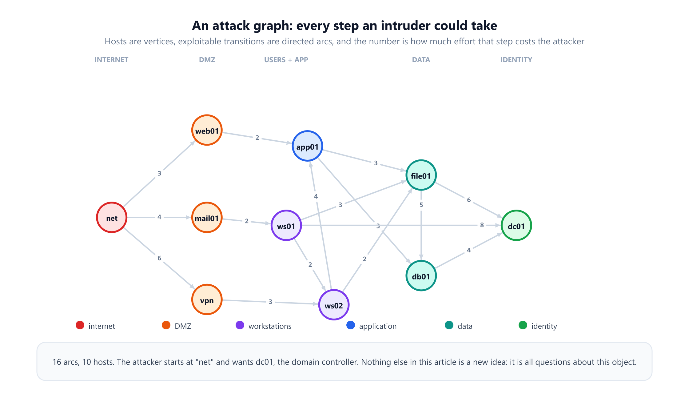
The running example is a small enterprise, deliberately ordinary. The internet reaches three exposed systems: a public web server, a mail gateway and a VPN concentrator. Behind them sit two workstations and an application server, then a file server and a database, and finally the domain controller, which is what the attacker wants.
| Zone | Hosts | Why it is in the model |
|---|---|---|
| Perimeter | web01, mail01, vpn | The three ways in from the internet |
| Users and application | ws01, ws02, app01 | Where footholds land and credentials live |
| Data | file01, db01 | The assets, and the trust they carry |
| Identity | dc01 | The objective: domain compromise |
Each of the sixteen arcs carries an effort score and a control cost. The effort scores say that exploiting the public web application costs 3, that an internal service call from the DMZ into the app tier costs 2, and that stealing cached domain admin credentials off a workstation costs 8, which is hard but not impossible. Those relative judgements are the model's only real input.
One structural note before any algorithm runs: this graph has no cycles, because every arc moves the attacker inward. Real attack graphs do have cycles, since an attacker can pivot back and forth, and every algorithm used below handles them. The acyclic case simply makes the worked examples easier to check by hand.
4. The easiest way in: shortest attack paths
The first question is the one a penetration tester answers by hand over a fortnight: what is the easiest route from the internet to the domain controller? With effort on the arcs it is a shortest path problem, and Dijkstra's algorithm answers it for every asset at once.
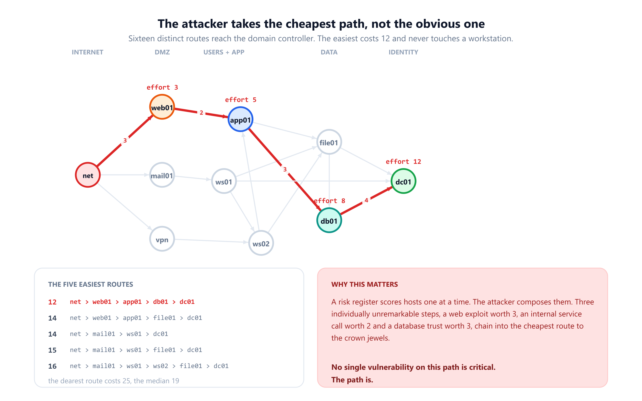
The answer is internet → web01 → app01 → db01 → dc01 at a total effort of 12. Read the steps: exploit the public web application (3), use the trusted internal service call into the app tier (2), reach the database the application is entitled to query (3), and abuse the database service account against the domain controller (4).
Two things about that result matter more than the number.
Not one of those four steps is individually alarming. A web application vulnerability rated 3 out of 10 does not top a risk register. Neither does a service call between two systems that are supposed to talk to each other. The route is dangerous as a composition, and no per-host severity score can express a composition. This is the fundamental argument for attack graphs, made by Phillips and Swiler in 1998 and repeated in every paper since.
The easiest route avoids the humans. Phishing is the most discussed initial access vector, and here the phishing route to the domain controller costs 14, not 12. The model does not say phishing is unimportant; it says that on this estate, with these scores, the server path is cheaper. Solving for the attacker's cheapest option rather than the defender's most feared option is precisely what the algorithm is for.
The same computation gives the effort to reach every other asset: web01 costs 3, app01 costs 5, the file server costs 8, the database costs 8. Those are the numbers to put in front of an audit committee that wants to know how far the perimeter really is from the crown jewels.
5. Sixteen ways in, and which host carries them
The cheapest path is one answer. Blocking it is not a strategy, because the attacker simply takes the next one. The useful question is how many routes exist and which assets they run through.
Enumerating every simple path from the internet to the domain controller on this graph gives 16 distinct routes, costing between 12 and 25 with a median of 18.5. Sixteen is a small number precisely because the example is small; a real estate with a few thousand hosts routinely has more attack paths than there are atoms worth counting, which is why enumeration is a teaching device and the metrics below are the production technique.
Counting how many of those routes pass through each host produces a ranking, and the ranking is not the one a perimeter report would give you.
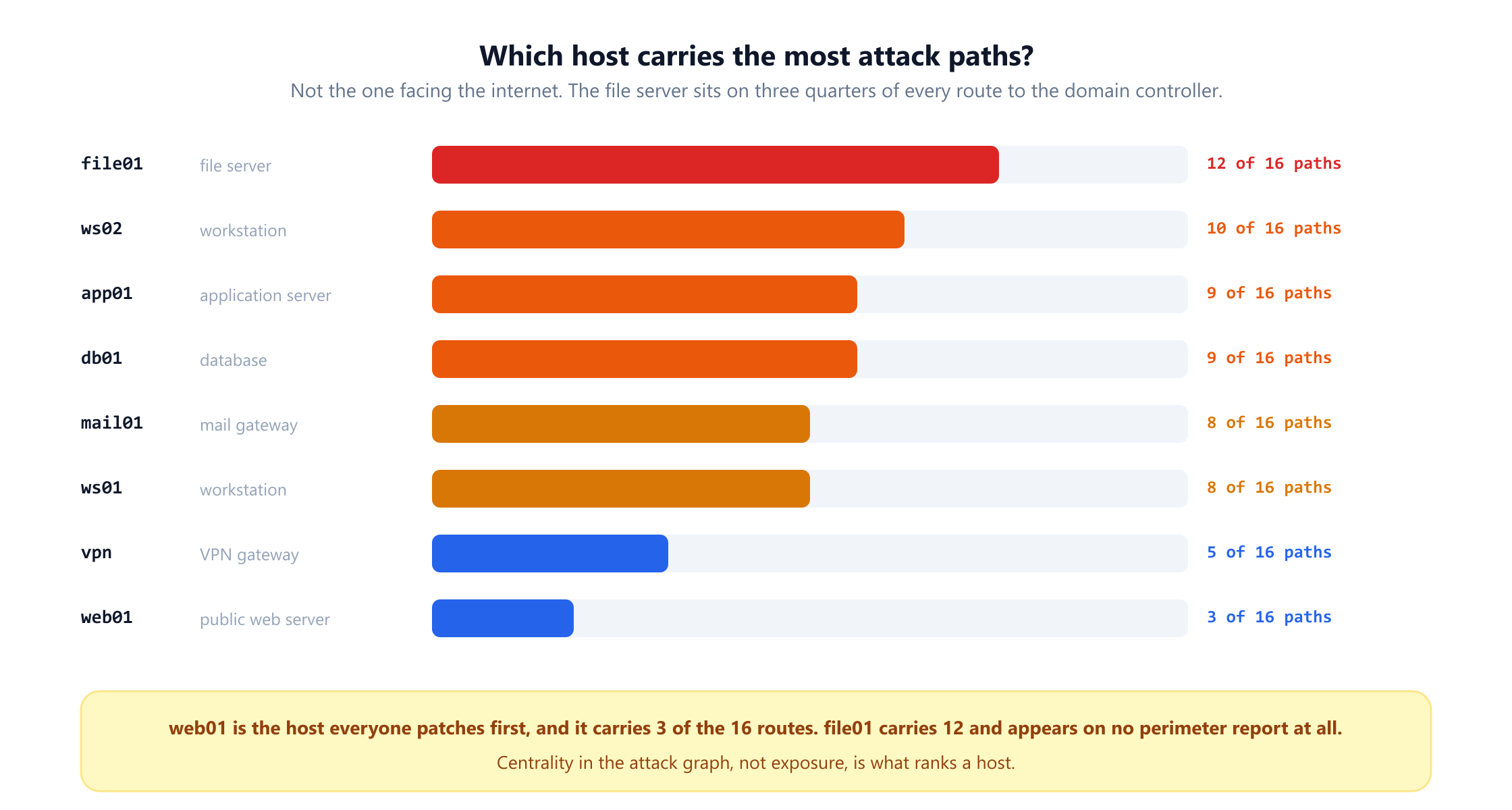
The file server sits on 12 of the 16 routes, three quarters of them. The public web server, the single most scrutinised machine in most organisations, sits on 3. Nothing about the file server would flag on an external scan: it is not exposed, it runs nothing exotic, and it exists to hold documents. It is critical because of where it sits in the graph, and only a graph can say so.
Enumeration is also where this approach stops scaling, and it is worth seeing why. Sixteen routes come out of ten hosts and sixteen arcs. Add a second file server that both workstations can reach and the count roughly doubles; a real estate with a few thousand machines and a flat internal network has a path count with more digits than anyone will ever read. The metrics below all avoid enumerating, which is what makes them usable on a real network.
This measure is a security-specific cousin of betweenness centrality, introduced by Freeman in 1977, which counts the fraction of shortest paths passing through a vertex. Betweenness over all pairs is the standard network-science measure and is computable in O(nm) by Brandes' algorithm. For defence, counting paths between the specific pair that matters, the attacker's entry and the asset you care about, is usually more actionable: it answers "if I harden one machine, how many routes does it disturb" rather than "how central is this in general".
Noel and Jajodia made the same argument for sensor placement in 2008: put your detection where the attack paths concentrate, not where the assets are most valuable, because the concentration points are where you get the most coverage per sensor.
6. Breaking every route: the minimum cut
Ranking hosts tells you where to look. The stronger question is what set of controls would break every route at once, and how little that could cost.
Give each arc the cost of the control that removes it, then compute the minimum cut between the internet and the domain controller. The max-flow min-cut theorem guarantees that the cheapest such set is exactly the minimum cut, and the algorithm returns it in polynomial time. The same machinery is covered in network flow, max-flow and min-cut.
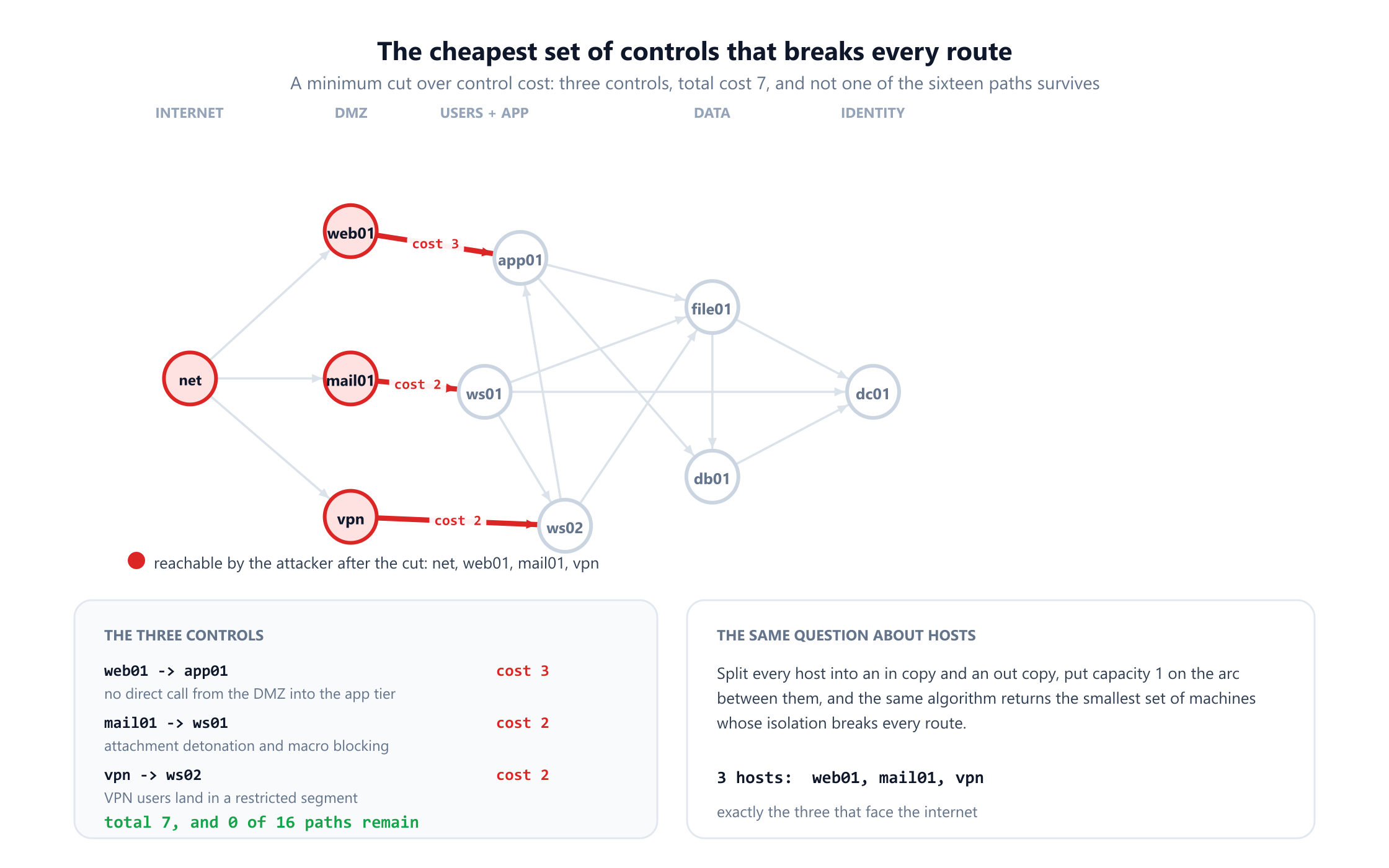
The answer is three controls totalling 7: stop the DMZ web server calling into the app tier (3), stop mail attachments executing on workstations (2), and land VPN users in a restricted segment rather than beside the workstations (2). Re-enumerating the paths after applying them returns zero.
Notice where the cut falls. Every one of the three controls sits at the boundary between the perimeter and the interior, and none of them touches the domain controller, the database or the file server. The instinct to harden the crown jewels first is not what the mathematics recommends: the cheapest complete fix is at the narrowest point of the graph, and here that is the first hop inward.
The same question about machines rather than links uses the node splitting trick. Replace each host with an "in" copy and an "out" copy joined by an arc of capacity 1, give the real arcs infinite capacity, and the minimum cut now counts hosts instead of links. The answer here is 3 hosts: web01, mail01 and vpn, which are exactly the three that face the internet. That is a reassuring sanity check on a small example and a genuinely useful computation on a large one, where the equivalent set is rarely obvious.
A caution about what is and is not polynomial. Finding the cheapest set of arcs or hosts to cut is a minimum cut, and it is fast. Finding the cheapest set of security measures is not the same problem: one patch may remove several arcs at once and one arc may need several measures, which turns it into a hitting set problem. Jha, Sheyner and Wing proved in 2002 that finding a minimum critical set of measures in an attack graph is NP-hard. Model the controls carefully, and know which of the two problems you are solving.
7. What one control actually buys
Budgets rarely fund three controls at once, so the practical question is which single one to buy first. Removing each arc in turn and re-solving gives an answer, and the answer is sobering.
| Control | Cost | Attacker effort | Routes remaining |
|---|---|---|---|
| Nothing (baseline) | 0 | 12 | 16 |
Block db01 → dc01 | 5 | 14 | 7 |
Block web01 → app01 | 3 | 14 | 13 |
Block internet → web01 | 4 | 14 | 13 |
Block app01 → db01 | 5 | 14 | 13 |
Block mail01 → ws01 | 2 | 12 | 8 |
Block ws01 → file01 | 3 | 12 | 14 |
The best single control raises the attacker's effort from 12 to 14. That is all. No individual measure on this network buys more than two points of difficulty, because the graph is richly connected and the attacker simply switches to the next-cheapest route. This is the quantitative version of a familiar security truth: defence in depth is not a slogan, it is a consequence of the fact that single cuts in a dense graph do very little.
The table also shows that the metric you choose changes the ranking. Blocking the mail gateway to workstation transition halves the number of routes, from 16 to 8, and leaves the attacker's easiest path completely untouched at 12. If your board reports "attack paths eliminated" you would call that control a success; if it reports "attacker effort" you would call it useless. Both numbers are real, they measure different things, and quoting only one is how security programmes end up optimising the wrong quantity.
The best value on this table is blocking the database's route to the domain controller: cost 5, effort up to 14, and routes down to 7. It is the only control that improves both metrics substantially, which no amount of intuition would have identified.
8. Blast radius: what one compromise reaches
Attack paths ask how an intruder gets in. The complementary question is what happens once they are in somewhere, and it is a plain reachability computation: from a compromised host, which assets can eventually be reached? One traversal per host answers it in linear time.
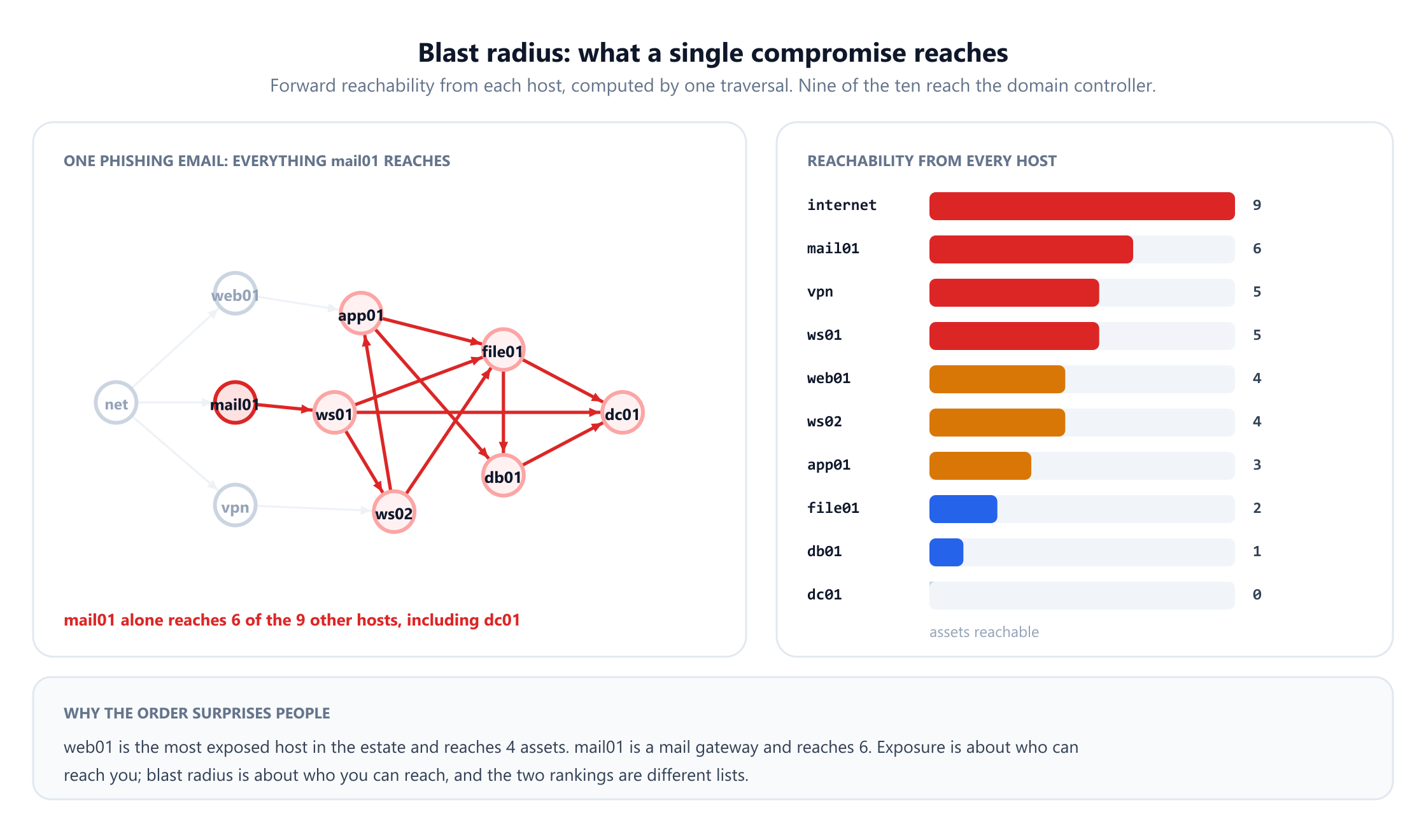
The ranking inverts the exposure ranking. The public web server, the most exposed machine in the estate, reaches 4 assets. The mail gateway reaches 6. A workstation reaches 5. Exposure measures who can reach you; blast radius measures who you can reach, and the two produce different priority lists from the same graph.
The number that should stop a meeting is this one: nine of the ten hosts can eventually reach the domain controller. Only the domain controller itself cannot, because nothing sits beyond it. On a real estate that figure is the single most useful output of the whole exercise, because it converts "we have flat networking" from an opinion into a measurement.
Blast radius is also what makes containment decisions tractable during an incident. When a host is confirmed compromised, the set of machines that need investigation is its forward reachable set, and the set that could have infected it is its backward reachable set, computed on the reversed graph. Both are one traversal, and both are far more precise than isolating a whole subnet on instinct.
9. How fast it spreads: the epidemic threshold
Ransomware and worms do not follow a single path; they spread. Modelling that needs a different question: given a network and an infection that propagates between neighbours and gets cleaned up at some rate, does it die out or take the estate?
The answer is one of the most useful results in network science, and it is exact. For a very broad class of spreading models, the tipping point depends on a single number: the largest eigenvalue of the adjacency matrix, written λ₁. An infection whose spread-to-cleanup ratio is below 1 / λ₁ dies out on its own; above it, it becomes endemic. Wang, Chakrabarti, Wang and Faloutsos proved this in 2003, and Chakrabarti and colleagues generalised it in 2008.
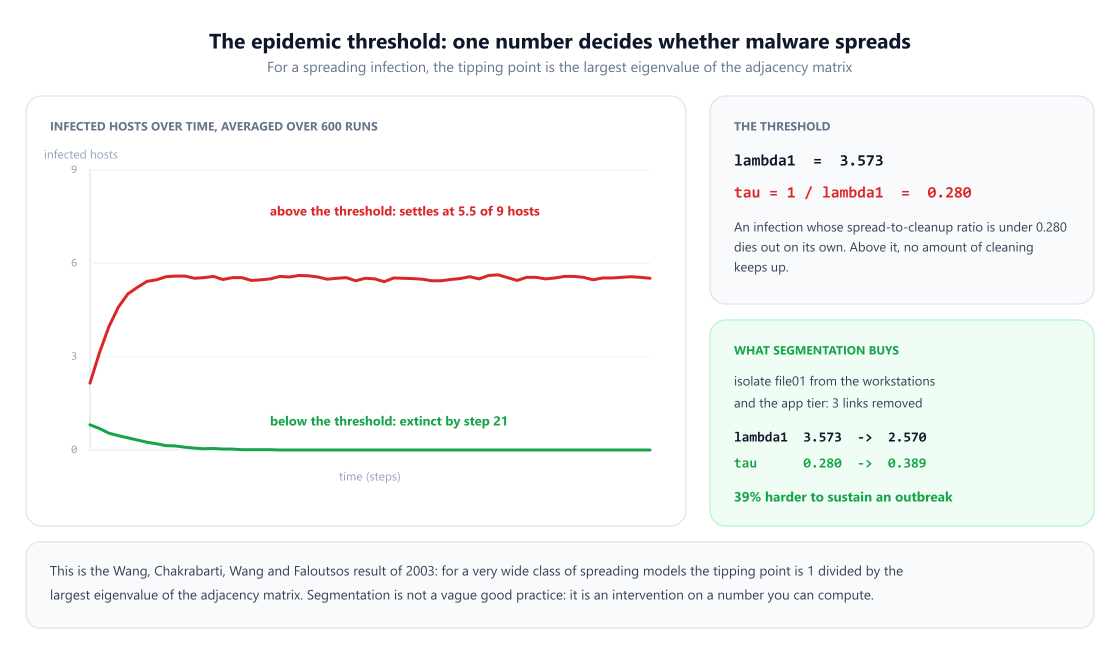
On the lateral movement graph here, nine hosts and thirteen links, λ₁ is 3.573, so the threshold is 0.280. Simulating an infection at 40% of that ratio, averaged over 600 runs, it is extinct by step 21. At four times the ratio it stabilises at 5.5 of the 9 hosts and stays there indefinitely. The threshold predicted both outcomes before either simulation ran.
What makes this operationally interesting is that λ₁ is something you can change. Isolating the file server from the workstations and the application tier removes three links and drops λ₁ from 3.573 to 2.570, raising the threshold from 0.280 to 0.389. That is a 39% larger margin: infections that would previously have taken hold now die out.
Two facts make the eigenvalue easier to reason about than it first looks. It always lies between the average degree and the maximum degree of the graph, which here means between 2.889 and 5, and 3.573 duly sits between them. And it is dominated by the densest part of the network, so the fastest way to lower it is to reduce the connectivity of the most connected host. That is exactly what the segmentation above does: the file server has degree 5, the highest in the estate, and cutting three of its links takes it to 2 and drops the maximum degree of the whole graph from 5 to 3. The most connected machine is the one to isolate, and degree is a one-line calculation you can run before touching any eigenvalue code.
This reframes segmentation. "Segment the network" is usually justified with a story; here it is an intervention on a computable quantity, with a before and an after. The lineage of the idea runs back to Kephart and White, who built directed-graph epidemiological models of computer viruses for IEEE Security and Privacy in 1991, and to Staniford, Paxson and Weaver, whose 2002 analysis of worm propagation showed how quickly the curve moves when the graph is dense.
10. Active Directory: the graph attackers already use
Everything so far has been a model built by a defender. The most consequential graph in enterprise security is one that already exists, that nobody deliberately designed, and that attackers have been querying for years: Active Directory.
An AD environment is a graph whether or not anyone draws it. Users are vertices, groups are vertices, computers are vertices, and the arcs are the relationships the directory already stores: member of, admin to, can reset password of, has a session on, owns, has generic write over. Every one of those relationships is a transition an attacker can use.
In 2016 Robbins, Vazarkar and Schroeder released BloodHound and gave the talk that named the technique, "Six Degrees of Domain Admin". Its insight is exactly the insight of this article: the individually harmless facts compose. A help desk group that can reset passwords for a group that contains a user who happens to have an active session on a server where a domain admin logged in last Tuesday is a four-hop path to total compromise, and no individual link in it looks like a misconfiguration.
What BloodHound does is collect those relationships and run a shortest path query against them. It is Dijkstra, on a graph nobody had thought to draw. The result changed defensive practice, because the paths it surfaced were both real and invisible to every other tool in use.
Three lessons transfer to any environment:
- The data already exists. Directory relationships, cloud IAM policies, Kubernetes role bindings and SaaS sharing permissions are all graphs sitting in a database, waiting to be queried as one.
- Sessions are arcs too. A logged-in session creates a temporary edge from that machine to that identity's privileges, which is why "who is logged in where" is a security question and not an inventory question.
- Cleanup is a graph edit. Removing one nested group membership can delete thousands of paths, and there is no way to see that without the graph.
11. Detection: provenance graphs and guilt by association
Attack graphs are about prevention. Two more graph techniques run on the detection side, and they use different graphs entirely.
Provenance graphs record what actually happened on a system: processes, files, sockets and the causal relations between them. A process reads a file, writes another, spawns a child, opens a connection. King and Chen introduced backtracking with their BackTracker system at SOSP in 2003: given a detection point, such as a suspicious file, walk backwards through the causal graph to find how it got there. Forward traversal from an entry point tells you the damage; backward traversal from a symptom tells you the root cause. Both are graph traversals over the same recorded structure.
The modern version correlates those flows against known attacker behaviour. HOLMES, published at IEEE Security and Privacy in 2019, maps suspicious information flows in a provenance graph onto the tactics and techniques of an attack lifecycle and raises an alert when the pattern of flows resembles an intrusion rather than ordinary activity. The engineering difficulty is scale: provenance graphs grow by millions of edges an hour on a single busy host, which makes efficient reduction and querying the entire research problem.
Guilt by association is the second technique, and it is graph inference rather than traversal. Build a bipartite graph of machines and files: a machine is connected to every file it has seen. Most files and machines are unlabelled, but a few are known good and a few are known bad. Belief propagation then spreads those labels along the edges, on the assumption that files appearing on many infected machines are suspicious and machines holding many bad files are compromised.
This is what Chau, Nachenberg, Wilhelm, Wright and Faloutsos built as Polonium in 2011, running over a graph of roughly 60 billion machine-file edges from Symantec telemetry, and reporting around 85% true positive detection. The technique matters because it needs no signature and no sandbox: a file nobody has ever analysed can be judged by the company it keeps. The same shape of computation, a bipartite graph plus label propagation, drives fraud detection in payments and abuse detection on social platforms.
12. The software supply chain graph
The last graph is the one your build system walks. A modern application declares a handful of direct dependencies, each of which declares its own, and the transitive closure routinely runs to hundreds or thousands of packages. That closure is a directed acyclic graph, and it is an attack surface.
The security question is a reachability question. If a package deep in the graph is compromised, which of your applications execute its code? That is forward reachability from the compromised node in the reverse dependency graph, and it is the query every organisation scrambles to answer in the first hour of a supply chain incident. Teams that maintain a software bill of materials answer it in seconds; teams that do not spend days grepping.
Two properties of the graph make this dangerous in ways a list would not reveal. Depth hides risk: a package you never chose, three levels below one you did, runs with the same privileges as your own code. Popularity concentrates it: the packages with the highest in-degree are the highest-value targets, because compromising one reaches thousands of downstream projects at once, which is precisely the pattern documented in the review of real open source supply chain attacks by Ohm, Plate, Sykosch and Meier in 2020.
The useful defensive metrics are graph metrics. Count the transitive closure size, not the direct dependency count. Rank dependencies by how many of your applications reach them. Watch for packages with a single maintainer and a large in-degree, which is exactly the risk profile that has produced several of the best known incidents. The technique is identical to the blast radius computation in section 8, run over a different graph.
13. What is easy, what is hard
Attack graph analysis is unusual among security techniques in having a clean complexity story, and knowing which side of the line a question falls on saves a great deal of wasted effort.
| Security question | Graph problem | Cost |
|---|---|---|
| Easiest route to an asset | Shortest path | O(m + n log n) |
| What can this compromise reach? | Reachability | O(n + m) |
| Cheapest set of links to cut | Minimum cut | Polynomial |
| Smallest set of hosts to isolate | Minimum vertex cut | Polynomial |
| Where does spread tip over? | Largest eigenvalue | Polynomial |
| Which hosts are choke points? | Betweenness centrality | O(nm) |
| Enumerate every attack path | All simple paths | Exponential in the worst case |
| Minimum set of security measures | Hitting set on the attack graph | NP-hard |
| Cheapest hardening under a budget | Network interdiction | NP-hard |
The pattern is the familiar one: questions about flow and connectivity are cheap, questions about which discrete things to change are expensive. Enumeration is the trap in the middle. It is intuitive, it is what every demonstration does, and the number of simple paths can grow exponentially with the size of the network, which is why serious tools compute metrics over the graph rather than listing its paths. Ammann, Wijesekera and Kaushik made exactly this argument in 2002 when they proposed a compact, monotonic representation that scales polynomially instead of enumerating.
One metric worth knowing by name is k-zero day safety, proposed by Wang, Jajodia, Singhal, Cheng and Noel in 2014. It asks how many distinct unknown vulnerabilities an attacker would need to reach an asset, which sidesteps the unanswerable question of how likely each individual exploit is. It is a graph distance under a different weighting, and it is a good example of the field's better instinct: measure structure, not probability.
14. Modelling mistakes
An attack graph that is wrong is worse than none, because it produces confident, specific, incorrect priorities. These are the failures that recur.
- Getting the arc direction wrong. A workstation mounting a share creates an arc into the share. Reversing it makes the file server look safe and the workstation look critical, and nothing about the output looks broken.
- Modelling hosts when the risk is identities. If the real transition is a credential that works in three places, an arc between two machines does not capture it. This is why the Active Directory graph in section 10 is a separate model and not a refinement of this one.
- Treating scores as measurements. The effort numbers are judgements. Trust the ordering, distrust the third decimal place, and test whether the conclusion survives perturbing the scores. If the recommended control changes when a 3 becomes a 4, say so.
- Forgetting that the graph is a snapshot. A laptop that joins the VPN adds arcs; a decommissioned server removes them; a temporary firewall exception during a migration can open a route that no diagram ever recorded. An attack graph is only as current as the inventory behind it.
- Enumerating paths on a real estate. It works beautifully on ten hosts and never finishes on ten thousand. Compute cuts, centrality and reachability instead, all of which are polynomial.
- Reporting a single metric. Section 7 showed a control that halves the number of attack paths and does not slow the attacker down at all. Publish attacker effort and route count together, or the programme will optimise whichever one is on the slide.
- Ignoring the arcs you cannot remove. Some transitions are the business: the application must query the database. The model should mark those as fixed, so the optimiser stops proposing controls that will never be approved.
15. From model to practice
Four things separate a diagram that impresses a meeting from a model that changes decisions.
Build the graph from data you already have. Firewall rule sets, cloud security group definitions, vulnerability scan output, Active Directory relationships and EDR telemetry all describe edges. A model assembled by hand in a workshop is out of date the week after the workshop; a model generated from configuration is regenerated nightly.
Start with reachability, not attack paths. The cheapest valuable result is the blast radius table from section 8, because it needs no exploit scoring at all, only connectivity. "Nine of our ten hosts can reach the domain controller" is a finding that lands, and you can produce it before anyone argues about CVSS.
Use the tools that exist. MulVAL, the scalable attack graph generator published by Ou, Boyer and McQueen in 2006, is still the reference implementation in research. BloodHound covers the identity graph. NetworkX or a graph database handles the analysis once the edges exist. None of the algorithms in this article needs to be written from scratch, and the graph chapters of any algorithms text cover the ones that do.
Re-solve rather than argue. Every claim in this article was a claim the model settled in milliseconds: that the easiest route avoids the workstations, that the file server carries four times the routes of the web server, that the best single control buys two points of effort, that segmentation raises the epidemic threshold by 39%. Intuition about networks is unreliable in exactly the cases that matter, and the whole value of building the graph is that you stop needing it.
16. Where to go next
The fastest way to internalise this material is to build a graph rather than read about one, and the barrier is lower than it looks. Ten hosts and sixteen arcs, which is all this article used, fit in a text file, and every result above came out of a few dozen lines of ordinary code.
A sensible order to learn the pieces: get comfortable with breadth first and depth first search, since reachability and blast radius are nothing more than a traversal with bookkeeping. Then shortest path algorithms, which give you the easiest-route analysis and, with negative logarithms on the arcs, the most-likely-route analysis too. Then max-flow and min-cut, which is the whole of sections 6 and 7 and the single most under-used result in defensive security.
After that the useful direction is structural rather than algorithmic: directed versus undirected graphs settles a surprising number of modelling arguments, and graph representation decides whether your analysis runs in a second or an hour once the estate is large. The complexity boundaries in section 13 are laid out more generally in graph algorithms and complexity.
If you would rather start from the security side, the shortest path to a real result is to export your Active Directory relationships and query them, because that graph already exists and nobody had to model it. The finding that follows is usually the same one this article ends with: the number of machines that can eventually reach the domain controller is far higher than anyone in the room expected.
17. Frequently asked questions
What is an attack graph?
+
A directed graph whose vertices are the states an intruder can occupy, usually hosts or host-and-privilege pairs, and whose arcs are the transitions between them: an exploitable service, a trust relationship, a reused credential. Weights on the arcs record how much effort each step costs, how likely it is to succeed, or how much the control that removes it would cost. Once the graph exists, the questions defenders ask become standard algorithms: shortest path for the easiest intrusion, minimum cut for the cheapest complete fix, reachability for blast radius.
Why is a graph better than a list of vulnerabilities?
+
Because breaches are compositions, and a list cannot express a composition. On the network in this article the easiest route to the domain controller is made of four individually unremarkable steps, none of which would reach the top of a severity-sorted list, and their combination is the cheapest intrusion available. A list also cannot tell you that the file server sits on three quarters of all routes while the internet-facing web server sits on under a fifth. Those are properties of the structure, not of any single host.
How do I find the cheapest way to block every attack path?
+
Put the cost of each mitigating control on the corresponding arc and compute the minimum cut between the attacker's starting point and the asset. The max-flow min-cut theorem guarantees the cheapest set of arcs that separates them is exactly that cut, and it is computed in polynomial time. To count hosts rather than links, split every host into an in copy and an out copy joined by an arc of capacity one and give the real arcs infinite capacity; the same algorithm then returns the smallest set of machines to isolate.
What is the epidemic threshold, and why does it matter for ransomware?
+
For a wide class of spreading models, an infection dies out on its own if its spread-to-cleanup ratio is below one divided by the largest eigenvalue of the network's adjacency matrix, and becomes endemic above it. That result is due to Wang, Chakrabarti, Wang and Faloutsos in 2003. It matters because the eigenvalue is something segmentation changes: on the network in this article, isolating the file server from the workstations and the app tier drops the eigenvalue from 3.573 to 2.570 and raises the threshold by 39%, turning outbreaks that would have taken hold into ones that fade.
What is BloodHound doing, mathematically?
+
Running shortest path queries on a graph built from Active Directory relationships. Users, groups and computers are vertices; membership, administrative rights, password reset rights, ownership and active sessions are arcs. The tool collects those relationships and finds routes from a low-privilege account to Domain Admin. The technique is ordinary graph search; the contribution was recognising that the directory already contains the graph, and that chains of individually reasonable permissions compose into total compromise.
Can attack graph analysis scale to a real network?
+
The analysis scales; naive enumeration does not. The number of simple attack paths can grow exponentially with the size of the network, so listing them is hopeless beyond toy examples. Everything else in this article is polynomial: shortest paths, reachability, minimum cuts, centrality and the eigenvalue are all comfortably computable on graphs with millions of edges. The standard research answer, from Ammann and colleagues in 2002 and the MulVAL generator in 2006, is to use a compact representation whose size grows polynomially and to compute metrics over it rather than enumerating paths.
Where do the effort scores come from, and what if they are wrong?
+
Usually from a scoring system such as CVSS exploitability, adjusted by someone who knows the estate. They are judgements rather than measurements, and the honest position is that the ordering is much more reliable than the values: you may not defend 3 against 4, but you can defend that a public web exploit is easier than stealing a domain admin credential. Test the conclusion by perturbing the scores. If the recommended control changes when one score moves by a point, report that instead of pretending the model is precise. Metrics such as k-zero day safety exist precisely to sidestep the scoring problem by counting distinct unknown vulnerabilities instead.
18. References
The papers that established these techniques, in chronological order.
- Ford, L. R. and Fulkerson, D. R. (1956). “Maximal flow through a network.” Canadian Journal of Mathematics, 8, 399–404.
- Freeman, L. C. (1977). “A set of measures of centrality based upon betweenness.” Sociometry, 40(1), 35–41.
- Kephart, J. O. and White, S. R. (1991). “Directed-graph epidemiological models of computer viruses.” Proceedings of the IEEE Symposium on Security and Privacy, 343–359.
- Phillips, C. and Swiler, L. P. (1998). “A graph-based system for network-vulnerability analysis.” Proceedings of the New Security Paradigms Workshop, 71–79.
- Ammann, P., Wijesekera, D. and Kaushik, S. (2002). “Scalable, graph-based network vulnerability analysis.” Proceedings of the 9th ACM Conference on Computer and Communications Security, 217–224.
- Sheyner, O., Haines, J., Jha, S., Lippmann, R. and Wing, J. M. (2002). “Automated generation and analysis of attack graphs.” Proceedings of the IEEE Symposium on Security and Privacy, 273–284.
- Jha, S., Sheyner, O. and Wing, J. (2002). “Two formal analyses of attack graphs.” Proceedings of the 15th IEEE Computer Security Foundations Workshop, 49–63.
- Staniford, S., Paxson, V. and Weaver, N. (2002). “How to own the Internet in your spare time.” Proceedings of the 11th USENIX Security Symposium, 149–167.
- King, S. T. and Chen, P. M. (2003). “Backtracking intrusions.” Proceedings of the 19th ACM Symposium on Operating Systems Principles, 223–236.
- Wang, Y., Chakrabarti, D., Wang, C. and Faloutsos, C. (2003). “Epidemic spreading in real networks: an eigenvalue viewpoint.” Proceedings of the 22nd International Symposium on Reliable Distributed Systems, 25–34.
- Ou, X., Boyer, W. F. and McQueen, M. A. (2006). “A scalable approach to attack graph generation.” Proceedings of the 13th ACM Conference on Computer and Communications Security, 336–345.
- Chakrabarti, D., Wang, Y., Wang, C., Leskovec, J. and Faloutsos, C. (2008). “Epidemic thresholds in real networks.” ACM Transactions on Information and System Security, 10(4), 1–26.
- Noel, S. and Jajodia, S. (2008). “Optimal IDS sensor placement and alert prioritization using attack graphs.” Journal of Network and Systems Management, 16(3), 259–275.
- Chau, D. H., Nachenberg, C., Wilhelm, J., Wright, A. and Faloutsos, C. (2011). “Polonium: tera-scale graph mining and inference for malware detection.” Proceedings of the SIAM International Conference on Data Mining, 131–142.
- Wang, L., Jajodia, S., Singhal, A., Cheng, P. and Noel, S. (2014). “k-zero day safety: a network security metric for measuring the risk of unknown vulnerabilities.” IEEE Transactions on Dependable and Secure Computing, 11(1), 30–44.
- Robbins, A., Vazarkar, R. and Schroeder, W. (2016). “Six degrees of Domain Admin.” DEF CON 24.
- Milajerdi, S. M., Gjomemo, R., Eshete, B., Sekar, R. and Venkatakrishnan, V. N. (2019). “HOLMES: real-time APT detection through correlation of suspicious information flows.” Proceedings of the IEEE Symposium on Security and Privacy, 1137–1152.
- Ohm, M., Plate, H., Sykosch, A. and Meier, M. (2020). “Backstabber's knife collection: a review of open source software supply chain attacks.” Detection of Intrusions and Malware, and Vulnerability Assessment (DIMVA), 23–43.