
Table of Contents
- 1. Representation is not an implementation detail
- 2. The running example
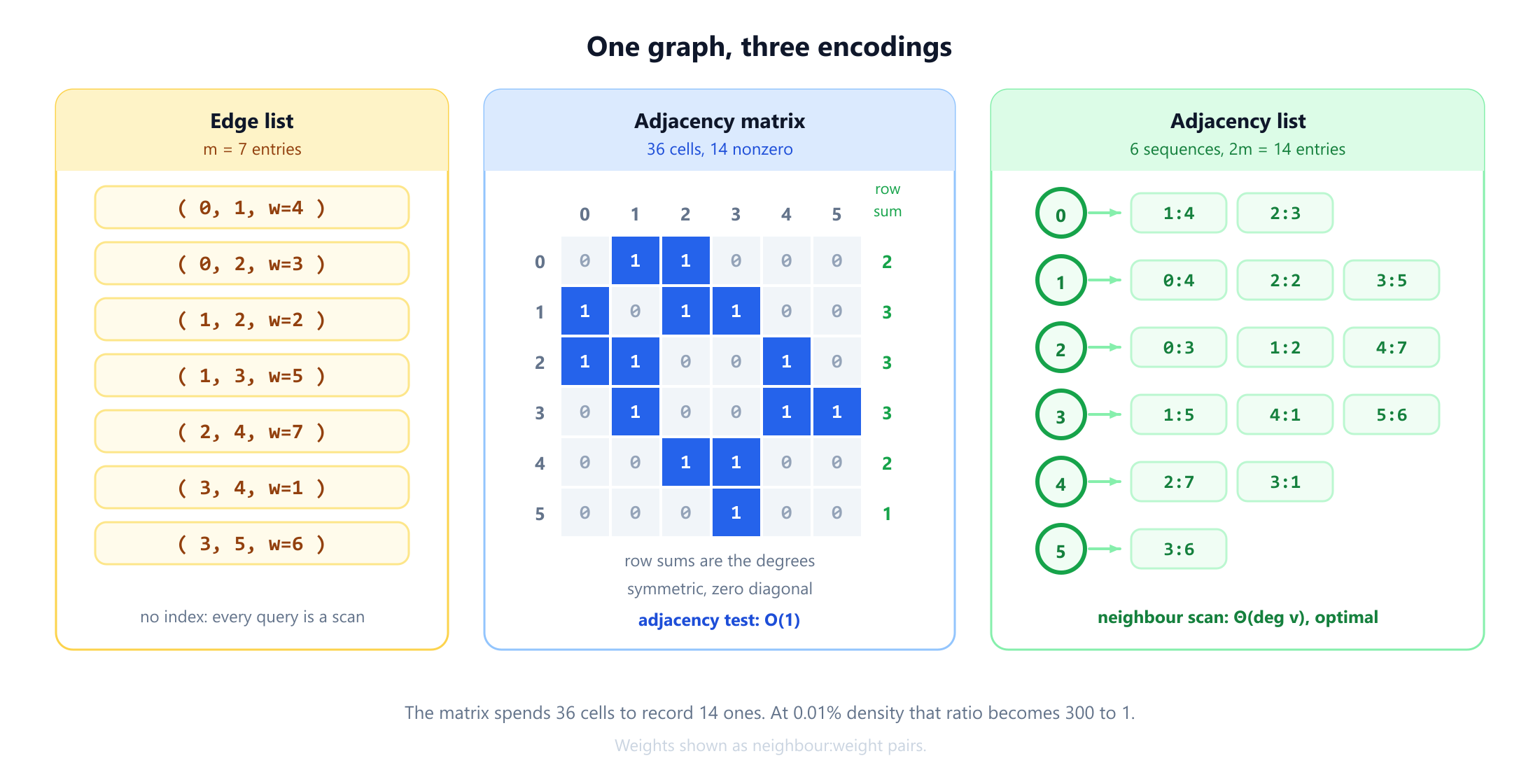
- 3. The edge list
- 4. The adjacency matrix
- 5. The adjacency list
- 6. What “sparse” actually means
- 7. Compressed sparse row
- 8. The incidence matrix
- 9. Direction, weight, multiplicity and loops
- 10. Algebraic representations
- 11. When the matrix wins
- 12. Graphs that change
- 13. Implicit graphs: storing nothing at all
- 14. Compressed and succinct representations
- 15. A decision procedure
- 16. Common mistakes
- 17. Glossary
- 18. Frequently asked questions
- 19. References
1. Representation is not an implementation detail
A graph is an abstract object: a set of vertices and edges, nothing more. A computer cannot store an abstract object. It stores bytes, and the choice of which bytes decides, before you write a single line of algorithm, what your program is capable of.
That claim is easy to state and easy to underestimate, so here is the sharpest version of it. Breadth-first search runs in O(n + m) time on an adjacency list and O(n2) time on an adjacency matrix. Same algorithm, same graph, same output. Only the storage differs. On a graph with a million vertices and fifty million edges, that is the difference between about 51 million operations and about a trillion: a factor of roughly 19,600. No amount of constant-factor tuning recovers that. The representation was the algorithm's asymptotic complexity all along.
The reason is simple once seen. Both versions of BFS do the same thing at each vertex: enumerate its neighbours. An adjacency list answers “who are v's neighbours?” in time proportional to how many there are. An adjacency matrix answers it by scanning a whole row of length n, most of which is zeros. Summed over all vertices, the list costs 2m and the matrix costs n2. This is exactly the observation that Hopcroft and Tarjan built their linear-time graph algorithms on in the early 1970s, and it is why the adjacency list became the default in every algorithms course since.
But the adjacency list is not always the answer, and treating it as the automatic default is its own mistake. Ask whether two given vertices are adjacent and the matrix answers in one memory access while the list scans a neighbour sequence. Multiply the graph by itself and the matrix hands you walk counts for free. Store a genuinely dense graph and the matrix uses less memory, not more. Run on a GPU and neither structure is what you want.
So the honest framing is not “which representation is best” but which question are you going to ask most often, and how big is the graph. This article works through the seven representations that matter in practice, derives the cost of each operation on each, and ends with a decision procedure. Every number about the example graph below was computed by script rather than asserted, and the arithmetic is reproduced so you can check it.
2. The running example
One small weighted graph carries the whole article. It is deliberately tiny enough to write out completely in every representation, and deliberately irregular enough that the representations look genuinely different.
V = {0, 1, 2, 3, 4, 5}

E = { {0,1}:4   {0,2}:3   {1,2}:2   {1,3}:5   {2,4}:7   {3,4}:1   {3,5}:6 }

n = 6      m = 7      degree sum = 14 = 2m
degrees    0:2   1:3   2:3   3:3   4:2   5:1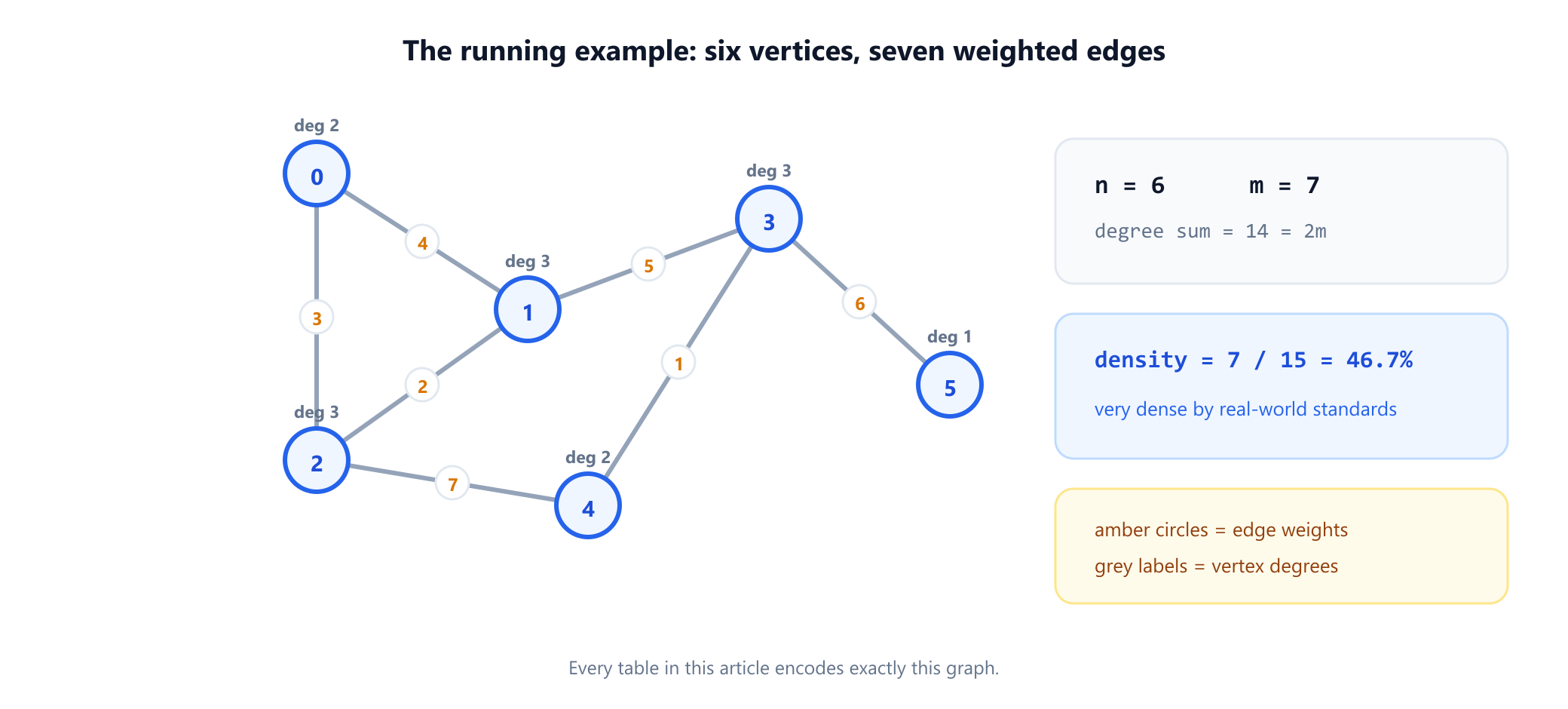
Two facts about it will keep coming back. Its neighbour sets, written in sorted order, are
0 → 1, 2
1 → 0, 2, 3
2 → 0, 1, 4
3 → 1, 4, 5
4 → 2, 3
5 → 3
and its density is 7 / 15 = 46.7%, since a simple graph on 6 vertices admits at most C(6,2) = 15 edges. That is very dense by real-world standards, which is a useful corrective: toy graphs in textbooks are almost always dense, and the intuitions they build about representation are almost always wrong for production data. We will fix that in section 6.
3. The edge list
The simplest representation is to write down the edges and stop.
edges = [ (0,1,4), (0,2,3), (1,2,2), (1,3,5), (2,4,7), (3,4,1), (3,5,6) ]An array of m triples. Space is Θ(n + m) if you also keep a vertex count, and Θ(m) if the vertex set is implicit in the edges. Nothing is precomputed, nothing is indexed.
The consequence is that almost every query is a full scan. “Are 1 and 4 adjacent?” requires walking all seven edges. “What are 3's neighbours?” requires walking all seven edges. Both are O(m), which is catastrophic if you do it inside a loop over vertices, because that turns into O(nm).
And yet the edge list is not a naive choice, because three important situations want exactly this shape:
- Algorithms that iterate over edges rather than vertices. Kruskal's algorithm sorts all edges by weight and considers them in order; it never asks for a neighbour list. Bellman-Ford relaxes every edge
n - 1times; again, pure edge iteration. For these, the edge list is not merely adequate, it is optimal, since any other representation would have to be flattened back into edge order. - Interchange and storage. Every graph file format on disk is an edge list, because it is the only representation that is order-independent, append-only and trivially parseable. When you download a dataset from SNAP or the DIMACS collections, you get an edge list, and your first step is to convert it.
- Streaming. If the graph does not fit in memory at all, an edge list is what arrives, one edge at a time, and the semi-streaming model of computation is built on the assumption that this is all you get.
The practical rule is that an edge list is a transport format and an iteration format, not a query format. Real systems read an edge list and immediately build something indexed. That conversion is the subject of section 7, and it is cheaper than people expect: a counting sort over vertex identifiers does it in O(n + m).
4. The adjacency matrix
Number the vertices 0 to n - 1 and build the n × n matrix A where A[u][v] = 1 if {u, v} is an edge and 0 otherwise. For the running example:
      0  1  2  3  4  5        row sum
  0 [ 0  1  1  0  0  0 ]         2
  1 [ 1  0  1  1  0  0 ]         3
  2 [ 1  1  0  0  1  0 ]         3
  3 [ 0  1  0  0  1  1 ]         3
  4 [ 0  0  1  1  0  0 ]         2
  5 [ 0  0  0  1  0  0 ]         1

36 cells, 14 of them nonzero
Three structural properties fall straight out, and each one is a usable check when debugging.
- The matrix of an undirected graph is symmetric.
A[u][v] = A[v][u]always, so half the storage is redundant. Directed graphs give up this symmetry, which is precisely what makes direction visible in the algebra. - The row sums are the degrees: 2, 3, 3, 3, 2, 1, matching the list in section 2. The total number of ones is
2m = 14, since each edge contributes two cells. - The diagonal is zero for a simple graph, because a nonzero diagonal entry is a loop.
What you buy is constant-time adjacency. Asking whether 1 and 4 are adjacent is one array read, A[1][4], independent of degree. No other representation in this article does that without hashing. What you pay is Θ(n2) space regardless of how many edges exist, and Θ(n) time to enumerate one vertex's neighbours regardless of how few it has.
That last cost is the one that bites. Vertex 5 has a single neighbour, but reading row 5 to discover this touches six cells. Scale that to a million vertices and finding the neighbours of a degree-one vertex touches a million cells. The O(n2) in matrix BFS is entirely this effect, accumulated.
The bit-packing refinement. If the graph is unweighted, each cell needs one bit, not one byte and certainly not one 32-bit integer. Packing rows into machine words cuts memory by a factor of 8 against a byte matrix and 32 against an int matrix, and it does something more interesting: it lets you operate on 64 neighbours per instruction. Intersecting two neighbourhoods, which is the inner loop of triangle counting and of many clique algorithms, becomes a word-wise AND over n/64 words rather than a loop over n entries. We return to this in section 11, because it is the main reason dense representations survive.
5. The adjacency list
Store, for each vertex, a sequence of its neighbours.
adj[0] = [ (1,4), (2,3) ]
adj[1] = [ (0,4), (2,2), (3,5) ]
adj[2] = [ (0,3), (1,2), (4,7) ]
adj[3] = [ (1,5), (4,1), (5,6) ]
adj[4] = [ (2,7), (3,1) ]
adj[5] = [ (3,6) ]
Space is Θ(n + m): one slot per vertex plus 2m = 14 neighbour entries for an undirected graph, or m for a directed one. Enumerating the neighbours of v costs Θ(deg(v)), which is optimal, since you cannot list k things in less than k time.
This is the representation that makes linear-time graph algorithms possible, and its adoption has a precise history. Tarjan's 1972 depth-first search paper and the Hopcroft and Tarjan companion algorithms of 1973 are explicit that the O(n + m) bounds depend on adjacency-list storage; the same procedures on a matrix are O(n2). Aho, Hopcroft and Ullman's 1974 textbook then made the list the standard presentation, and it has been the default in traversal code ever since.
The cost is that adjacency testing is no longer constant. To answer “are 1 and 4 adjacent?” you scan adj[1], three entries, and find nothing. In general that is O(deg(u)), or O(min(deg(u), deg(v))) if you are careful enough to scan the shorter list. On a graph with a few very high-degree vertices, which is what every social or web graph looks like, that minimum can still be millions.
The neighbour ordering question. Nothing in the definition says the neighbour sequences must be sorted, and most code leaves them in insertion order. Sorting them costs O(m log m) once and buys two things: binary-searchable adjacency in O(log deg(u)), and linear-time neighbourhood intersection by merge, which is what fast triangle-counting implementations rely on. If you intersect neighbourhoods at all, sort.
The implementation trap. The textbook picture of an adjacency list is an array of linked lists, and the textbook picture is bad advice on modern hardware. A linked list dereferences a pointer per neighbour, and each dereference is a potential cache miss costing on the order of a hundred cycles. A vector<vector<int>> is better, since each vertex's neighbours are contiguous, but it still scatters n separately allocated blocks across the heap and pays a per-vertex allocation header. The fix is section 7.
Hash-based variants. Replacing each neighbour sequence with a hash set gives expected O(1) adjacency testing while keeping Θ(n + m) space, which looks like the best of both. In practice the constant is unkind: a hash set costs several times the memory of a packed array of integers, destroys iteration locality, and makes the neighbour scan, which is the operation you actually do most, meaningfully slower. Use it when adjacency queries genuinely dominate traversal, and measure rather than assume.
6. What “sparse” actually means
Everything above turns on one word. A graph is sparse when m is close to n and dense when m is close to n2, and the practical dividing line is the density
density = m / C(n,2) = 2m / (n(n-1))which is the fraction of possible edges that exist. The running example sits at 7/15 = 46.7%, which is enormously dense. Real graphs are not like this. A social network with a million users and fifty million friendships, an average of 100 friends each, has density 1.0 × 10⁻⁴: one hundredth of one percent. Road networks are worse still, with average degree under 3 because intersections have a bounded number of roads. The web graph, citation graphs, protein interaction networks and dependency graphs are all in the same regime.
Here is what that costs, computed for exactly that million-vertex graph:
| Representation | Formula | Bytes for n = 106, m = 5 × 10⁷ |
|---|---|---|
| Adjacency matrix, one byte per cell | n2 | 931 GiB |
| Adjacency matrix, one bit per cell | n2 / 8 | 116 GiB |
vector<vector<int>> adjacency list | ≈ 40n + 8m | 420 MiB |
| Compressed sparse row | 8(n+1) + 8m | 389 MiB |
The matrix is roughly 300 times larger than the sparse structures even when packed down to single bits, and it does not fit in the memory of any ordinary machine. This is not a marginal preference. It is the difference between a program that runs and one that cannot be started.
The crossover is worth knowing precisely. A bit-packed matrix costs n2/8 bytes; a sparse structure storing a 4-byte target per directed arc costs about 8m bytes. The matrix wins when n2/8 < 8m, that is when m > n2/64, which corresponds to a density above roughly 3.1%. Above that, use a matrix; below it, do not. Almost every graph you will meet outside of small combinatorial search problems is below it by three orders of magnitude.
The full operation-by-operation comparison, with d written for the degree of the vertex involved:
| Operation | Edge list | Adjacency matrix | Adjacency list | CSR |
|---|---|---|---|---|
| Space | Θ(n + m) | Θ(n2) | Θ(n + m) | Θ(n + m) |
Is u adjacent to v? | O(m) | O(1) | O(d) | O(d), or O(log d) sorted |
List the neighbours of u | O(m) | Θ(n) | Θ(d) | Θ(d), contiguous |
Degree of u | O(m) | Θ(n) | O(1) | O(1) |
| Iterate over all edges | Θ(m) | Θ(n2) | Θ(n + m) | Θ(n + m) |
| Add an edge | O(1) | O(1) | O(1) amortised | Θ(n + m) rebuild |
| Delete an edge | O(m) | O(1) | O(d) | Θ(n + m) rebuild |
| BFS or DFS | O(nm) | Θ(n2) | Θ(n + m) | Θ(n + m), faster constant |
The table in essentially this form is the standard presentation, going back to Aho, Hopcroft and Ullman and reproduced in the graph chapter of Cormen, Leiserson, Rivest and Stein. Read it as a statement about which question you ask, not about which row is best. The only cell where the matrix is uniquely strong is adjacency testing, and the only cells where the edge list is strong are whole-edge iteration and appending. Everything else belongs to the sparse indexed structures.
7. Compressed sparse row
The representation that production graph code actually uses is not the array-of-vectors adjacency list. It is compressed sparse row, borrowed wholesale from sparse linear algebra, where it has been standard since Gustavson's work in the early 1970s and is documented in Duff, Erisman and Reid as the canonical sparse storage scheme. Graph people sometimes call it the forward star representation, or simply a flattened adjacency list.
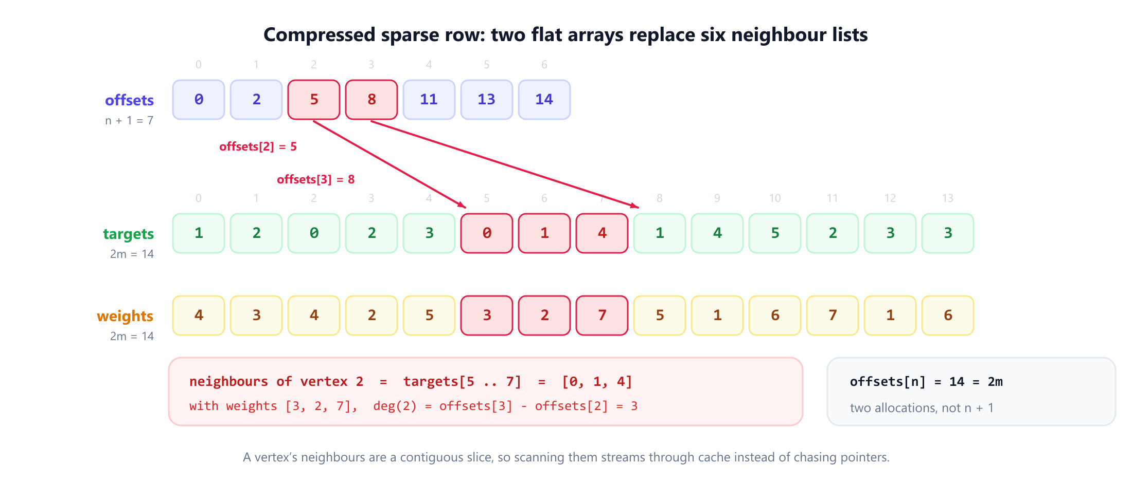
The idea is to concatenate all the neighbour sequences into one array and keep a second array recording where each vertex's slice begins.
offsets = [ 0, 2, 5, 8, 11, 13, 14 ]                       length n + 1 = 7
targets = [ 1, 2, 0, 2, 3, 0, 1, 4, 1, 4, 5, 2, 3, 3 ]     length 2m  = 14
weights = [ 4, 3, 4, 2, 5, 3, 2, 7, 5, 1, 6, 7, 1, 6 ]     length 2m  = 14
The neighbours of vertex v are targets[offsets[v] .. offsets[v+1] - 1]. For vertex 2 that is positions 5 through 7, giving neighbours [0, 1, 4] with weights [3, 2, 7], which matches adj[2] exactly. Degree comes for free as offsets[v+1] - offsets[v], recovering 2, 3, 3, 3, 2, 1 without touching the target array at all.
Asymptotically this is identical to an adjacency list. In practice it is substantially faster, for four reasons that have nothing to do with big-O:
- Locality. A vertex's neighbours occupy consecutive bytes, so scanning them streams through cache lines instead of chasing pointers. The hardware prefetcher can see the access pattern and stay ahead of it.
- No per-vertex allocation. Two allocations replace
n + 1of them. On the million-vertex example that removes about 38 MiB of headers and, more importantly, removes a million opportunities for the neighbour blocks to be scattered. - Trivially serialisable. The whole structure is two integer arrays, so it can be memory-mapped from disk, sent over a network, or handed to a GPU with no pointer fixing.
- Index compression. Since
targetsholds vertex identifiers, a graph with fewer than 232 vertices needs only 4 bytes per entry, and one with fewer than 216 needs 2. The offsets array does need 64-bit entries once2mexceeds 231, which is a real and frequently made mistake at billion-edge scale.
Building CSR from an edge list is O(n + m) and does not require sorting. Count the degree of every vertex in one pass, prefix-sum the counts into offsets, then make a second pass placing each edge into its slot using a moving cursor per vertex. This is a counting sort by source vertex, and it is the standard ingestion path in every serious graph library.
The price is rigidity. Inserting one edge shifts every subsequent entry in targets, so the structure is effectively immutable: you rebuild it in Θ(n + m) rather than update it. That is a fine trade when the graph is loaded once and queried many times, which describes most analytics workloads, and a bad one when the graph changes constantly. Section 12 deals with the second case.
8. The incidence matrix
The third classical matrix indexes vertices against edges rather than against vertices. Label the seven edges e1 through e7 in the order they were listed, and set B[v][e] = 1 when v is an endpoint of e:
       e1 e2 e3 e4 e5 e6 e7
   0 [  1  1  0  0  0  0  0 ]
   1 [  1  0  1  1  0  0  0 ]
   2 [  0  1  1  0  1  0  0 ]
   3 [  0  0  0  1  0  1  1 ]
   4 [  0  0  0  0  1  1  0 ]
   5 [  0  0  0  0  0  0  1 ]

column sums all 2      row sums 2,3,3,3,2,1 = degrees
The shape is n × m, so space is Θ(nm), which is worse than the adjacency matrix for any graph with more edges than vertices. Nobody stores a graph this way for computation. The incidence matrix earns its place for a different reason: it is the bridge between graph theory and linear algebra.
Two identities make the point. For the unsigned matrix above, B BT = A + D, where D is the diagonal matrix of degrees. Substituting the running example's numbers confirms it exactly. If instead you orient each edge arbitrarily and write -1 at its tail and +1 at its head, the signed incidence matrix Bs satisfies
B_s B_s^T = D - A = L, the Laplacianindependently of which orientation you chose. That identity is the reason the Laplacian is positive semidefinite, and it is the entry point to spectral graph theory. Diestel develops this line further, using the incidence matrix to define the cycle space and the cut space of a graph, two vector spaces over the field of two elements whose dimensions are m - n + c and n - c for a graph with c components. The incidence matrix is also the natural setting for flow problems: the constraint matrix of a network flow linear program is the signed incidence matrix, and its total unimodularity is what guarantees that the linear program has integer optimal solutions.
One further note. The incidence matrix handles multigraphs more gracefully than the adjacency matrix does, since parallel edges are simply distinct columns rather than a count crammed into one cell. Hypergraphs, where an edge may join more than two vertices, have no sensible adjacency matrix at all but a perfectly natural incidence matrix with column sums greater than two. If you ever need to generalise past ordinary graphs, this is the representation that generalises.
9. Direction, weight, multiplicity and loops
Everything so far assumed a simple undirected graph. Four common departures change what each representation must do, and the differences are where implementation bugs cluster.
Direction. In a directed graph the adjacency matrix stops being symmetric, and A[u][v] = 1 means an arc from u to v only. The adjacency list stores each arc once instead of twice, so the neighbour arrays hold m entries rather than 2m. That halving is the single most common source of off-by-a-factor-of-two memory estimates.
The real complication is that a directed graph has two neighbourhoods. adj[v] gives successors; predecessors require either scanning the entire structure or storing a second copy with every arc reversed. Sparse linear algebra calls that second copy compressed sparse column, and any algorithm that walks backwards, including reverse reachability, Kosaraju's strongly connected components procedure and backward Dijkstra in bidirectional search, needs it. Budget for two structures, not one.
Weight. Weights can live in the matrix cells directly, replacing the 1 with the weight. The subtlety is what a non-edge becomes: 0 is a legitimate weight, so a 0 cell is ambiguous. The convention is to store ∞ for absent edges in shortest-path settings, which is exactly what Floyd-Warshall assumes on entry, and 0 in flow settings where a zero-capacity arc and an absent arc really are the same thing. Pick one deliberately. In sparse structures the weight goes in a parallel array indexed identically to targets, as in the CSR listing above, which keeps the two in lockstep and preserves locality. Storing pairs interleaved instead is also fine and sometimes better; storing weights in a separate hash map keyed by edge is almost always worse.
Multiplicity. Parallel edges break the adjacency matrix's basic premise, since a cell holds one value. The usual repair is to store the multiplicity as an integer count, which works for counting problems but discards per-edge data such as distinct weights or identifiers. Adjacency lists take multi-edges without complaint: the same neighbour simply appears more than once. If you need per-edge attributes on a multigraph, store edge identifiers in the neighbour arrays and keep the attributes in a separate edge table indexed by those identifiers, which is what most graph databases do.
Loops. A loop at v puts a nonzero on the diagonal. The convention that catches people out is that in an undirected graph a loop contributes 2 to the degree of v, so the standard undirected adjacency matrix stores A[v][v] = 2 for a single loop in order to keep the row-sum-equals-degree identity true. Plenty of code stores 1 instead and then quietly reports wrong degrees. In an adjacency list the same question becomes whether v appears once or twice in its own neighbour sequence, and the honest answer is that you must decide and document it, because both conventions exist in the literature.
10. Algebraic representations
Once a graph is a matrix, matrix operations mean something. This is not a curiosity; it is the basis of an entire style of graph computation.
Powers of the adjacency matrix count walks. The entry Ak[u][v] is exactly the number of walks of length k from u to v, which follows by induction from the definition of matrix multiplication. On the running example:
A^2 =  [ 2  1  1  1  1  0 ]
       [ 1  3  1  0  2  1 ]
       [ 1  1  3  2  0  0 ]
       [ 1  0  2  3  0  0 ]
       [ 1  2  0  0  2  1 ]
       [ 0  1  0  0  1  1 ]
Read off A2[1][4] = 2: there are two length-2 walks from 1 to 4, namely 1→2→4 and 1→3→4. Check it against the picture. The diagonal A2[v][v] is 2, 3, 3, 3, 2, 1, which is the degree sequence again, because a length-2 walk from v to itself is a step out to a neighbour and back. Going one power further, trace(A3) = 6, and dividing by 6 gives one triangle, which brute force confirms is {0, 1, 2}. The division by 6 counts the three starting points and two directions of each triangle.
The Laplacian. Define L = D - A:
L =  [  2 -1 -1  0  0  0 ]
     [ -1  3 -1 -1  0  0 ]
     [ -1 -1  3  0 -1  0 ]
     [  0 -1  0  3 -1 -1 ]
     [  0  0 -1 -1  2  0 ]
     [  0  0  0 -1  0  1 ]
Every row sums to zero, so the all-ones vector is in the kernel and L is singular. Kirchhoff's matrix-tree theorem says that deleting any one row and the matching column and taking the determinant counts the graph's spanning trees. All six cofactors of the matrix above equal 11, and enumerating all C(7,5) = 21 five-edge subsets and testing each for acyclicity finds exactly 11 spanning trees. The theorem is not an approximation; it is an identity, and it turns a counting problem that looks exponential into one determinant.
The Laplacian's eigenvalues carry more. The multiplicity of the eigenvalue 0 is the number of connected components. The second smallest eigenvalue, Fiedler's algebraic connectivity, measures how hard the graph is to disconnect, and the sign pattern of its eigenvector gives a usable graph bisection. This is the machinery behind spectral clustering and behind a large part of Chung's spectral graph theory.
Graphs as linear algebra over semirings. The deepest version of this idea is that many graph algorithms are matrix operations, once you change the arithmetic. Replace (+, ×) with (min, +) and matrix multiplication becomes shortest-path relaxation, so An-1 over the min-plus semiring is the all-pairs shortest-path matrix. Replace it with (OR, AND) and it becomes reachability. Breadth-first search from a source is repeated multiplication of a sparse frontier vector by the adjacency matrix over a boolean semiring. Kepner and Gilbert set this out systematically, and it is the specification the GraphBLAS standard implements. The payoff is practical: expressing an algorithm as sparse matrix-vector products lets it inherit decades of tuned parallel linear algebra, which is how many GPU graph frameworks are built.
11. When the matrix wins
Given section 6, it would be easy to conclude that adjacency matrices are a teaching device. They are not, and it is worth being precise about the four situations where the matrix is the right answer.
Small n. If n is a few hundred, n2 is a few tens of thousands of cells and the memory argument evaporates. Floyd-Warshall computes all-pairs shortest paths in Θ(n3) time and Θ(n2) space on a matrix, with a three-line inner loop and near-perfect cache behaviour; for n in the hundreds it routinely beats running Dijkstra n times on a sparse structure, despite the worse asymptotics. Competitive programming and operations research are full of this regime.
Genuinely dense graphs. Above the roughly 3.1% density crossover computed earlier, the matrix is smaller as well as faster. Complement graphs, similarity graphs with a permissive threshold, and constraint graphs from scheduling problems land here regularly.
Bitset parallelism. This is the strongest argument. Pack each matrix row into machine words and set operations on neighbourhoods become word-parallel. Transitive closure via the Four Russians technique, introduced by Arlazarov, Dinic, Kronrod and Faradzev in 1970, computes reachability in O(n3 / log n) by precomputing results for blocks of bits; the same trick with plain 64-bit words gives a very large constant-factor win with almost no code. Triangle counting, maximum clique via branch and bound, and Boolean matrix products all lean on this. A sparse structure simply cannot do 64 adjacency tests in one instruction.
Access to fast matrix multiplication. Some graph problems reduce to matrix multiplication and inherit its exponent. Seidel's algorithm computes all-pairs shortest paths in an unweighted undirected graph in O(nω log n) time by repeated squaring of the adjacency matrix, where ω is the matrix multiplication exponent. Alman and Vassilevska Williams brought ω below 2.3729 in 2021, and subsequent refinements have pushed it slightly lower still. These bounds are largely theoretical, since the algorithms achieving them have constants that make them impractical, but the reduction is real and it exists only because the graph is a matrix.
12. Graphs that change
Every structure above was described as if the graph were fixed. Many are not, and update cost is a dimension the standard comparison table underplays.
The clean cases are the extremes. An adjacency matrix supports both insertion and deletion in O(1), since both are a single cell write; its problem was never update speed. An edge list appends in O(1) but deletes in O(m), because it must find the edge first. CSR does neither: any structural change rebuilds the whole thing in Θ(n + m).
Adjacency lists sit in between and reward a little care. Appending a neighbour to a dynamic array is O(1) amortised. Deleting is O(deg(u)) to locate the entry, but only O(1) to remove it once found, provided you swap the last element into the hole rather than shifting everything down. If you also need to delete the reverse copy in an undirected graph, store each entry's position in its twin so the second deletion is O(1) too, which is exactly what the classic array-based edge representation with paired indices does.
Three patterns cover most real needs:
- Batch and rebuild. Accumulate updates in a small side buffer, answer queries against CSR plus buffer, and rebuild CSR when the buffer grows past a threshold. A rebuild costs
Θ(n + m), so spreading it overΘ(m)updates isO(1)per update whenevermis at leastn, which covers essentially every real graph. This is what most analytics systems do, and it is usually enough. - Tombstoning. Mark deleted entries rather than removing them, and compact periodically. Removing the entry becomes
O(1)once it has been found, and no other entry moves, so indices into the neighbour arrays stay valid. Locating the entry is stillO(deg(u))unless you already hold a handle to it, and every later scan has to skip dead entries. - Genuinely dynamic structures. When updates and connectivity queries interleave and both must be fast, the data structure literature has answers. Link-cut trees and Euler tour trees maintain a changing forest in logarithmic time per operation, and general dynamic connectivity on arbitrary graphs is built on top of them, at
O(log2 n)amortised per update. These are considerably more intricate than anything above, and you should reach for them only when the batch-and-rebuild pattern has been measured and found wanting.
One warning specific to hardware. A structure that is fast in the asymptotic table can be slow in practice because updates fragment it. An adjacency list that has grown by a million individual insertions has its neighbour blocks scattered across the heap in allocation order, and a subsequent traversal pays for that scattering on every vertex. Periodically rebuilding into CSR is often worth it purely to restore locality, even when no asymptotic bound changes.
13. Implicit graphs: storing nothing at all
There is one more representation, and it is the one people forget exists: do not store the graph.
An implicit or procedural graph is defined by a function. Instead of a data structure you supply a successor routine that, given a vertex, generates its neighbours on demand. Nothing is materialised until it is visited.
This is not a fringe technique. It is how essentially all of state-space search works:
- Puzzle and game state spaces. The graph of Rubik's cube configurations has about 4.3 × 10¹⁹ vertices. Storing it is not a question of engineering effort: one bit per state is already more than five exabytes, and the arcs, at eighteen per state, would run past six zettabytes. Its successor function, apply one of the eighteen face turns, is a dozen lines of code. Search algorithms work perfectly well on it.
- Planning and model checking. The reachable state graph of a concurrent program is generated by executing transitions. Explicit-state model checkers store only the visited set, never the edges.
- Geometric and grid graphs. A pathfinding grid has an obvious successor function, four or eight offsets with a bounds and obstacle check. An adjacency list for a 4096 by 4096 grid with eight-way movement holds 134 million entries, every one of which a two-line function reproduces exactly. This matters directly for A* on grids.
The consequences are worth stating plainly. Space drops from Θ(n + m) for the graph to Θ(|visited|) for the search, which is what makes the technique viable at all. In exchange you lose everything that requires seeing the whole graph: you cannot count edges, compute a degree distribution, or run any algorithm that iterates over all vertices. You also cannot cheaply ask for predecessors unless you write a second function for them, and regenerating a neighbourhood costs CPU every time instead of a memory read, which can be the more expensive option for a heavily revisited region.
Implicit representation is also what licenses the memory-bounded search family. Iterative deepening A* keeps only the current path rather than an open list, trading repeated regeneration for linear space, and it is only sensible because regeneration is possible at all.
14. Compressed and succinct representations
At web scale, even CSR is too large, and two distinct research lines attack that.
Exploiting structure. The WebGraph framework of Boldi and Vigna is the standard reference here. It observes that if you order web pages by URL, pages from the same site end up with nearly identical outlink sets, and their target lists are close together numerically. Encoding each list as a reference to a similar earlier list plus a small correction, then gap-encoding the remaining targets with a variable-length code, brings the web graph down to a few bits per link, an order of magnitude better than raw 32-bit identifiers. The technique is entirely dependent on a good vertex ordering, which is the general lesson: compression on graphs is mostly a relabelling problem. Blandford, Blelloch and Kash proved a complementary result for separable graphs, which includes planar graphs and most meshes, showing that a separator-based ordering gives O(n)-bit representations that still answer an adjacency query in constant time.
Succinct data structures. A different tradition asks for representations whose size approaches the information-theoretic minimum while still answering queries without decompression. Jacobson's 1989 work introduced the rank and select primitives that make this possible, and Munro and Raman extended it to trees and other structures. A rooted tree on n nodes needs about 2n bits rather than the n pointers a naive encoding spends, and navigation still runs in constant time. For a graph the general problem is harder, but the framing is the right one: the number of distinct labelled graphs on n vertices with m edges gives a lower bound of roughly m log(n2/m) bits, and how close a representation gets to that is a meaningful way to judge it.
Neither line is something to reach for by default. Both cost query time, both cost implementation complexity, and both are worth it only when the graph genuinely does not fit. The practical intermediate step, and the one most people should try first, is simply renumbering the vertices so that neighbours have nearby identifiers. That alone improves cache behaviour on ordinary CSR measurably, and it costs one breadth-first traversal.
15. A decision procedure
Collapsing everything above into something usable at a keyboard:
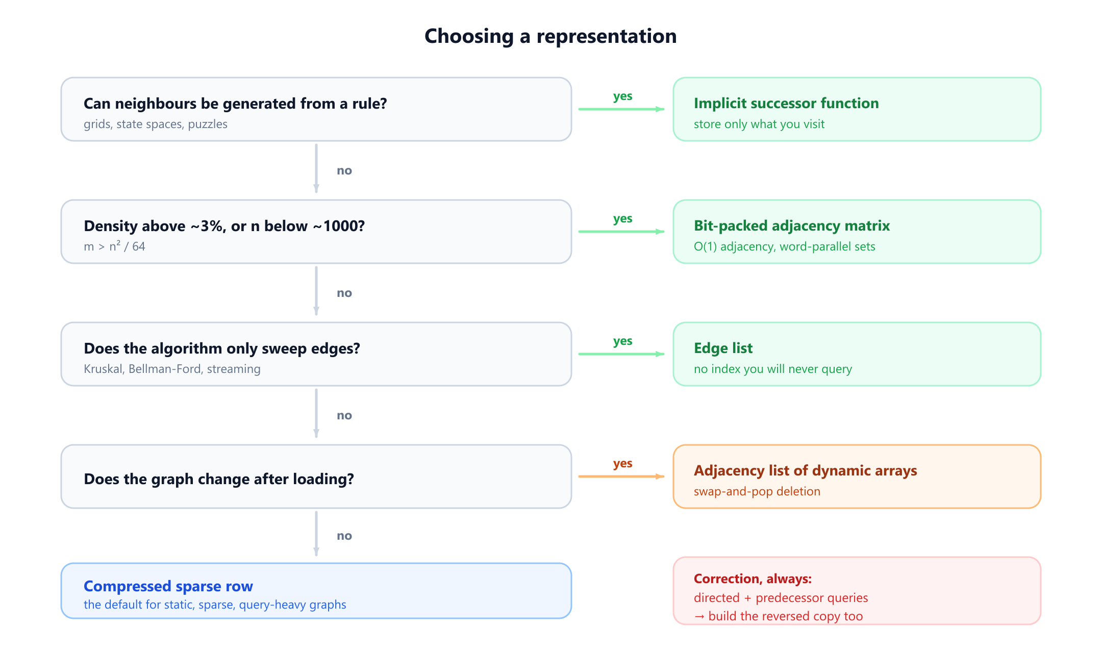
- Can you generate neighbours from a rule? If the graph is a state space, a grid, or anything procedurally defined, use an implicit representation and store only what you visit.
- Is the graph dense, or is
nsmall? Above about 3% density, or below roughly a thousand vertices, use a bit-packed adjacency matrix. You get constant-time adjacency and word-parallel set operations, and above the density crossover, less memory as well. Below it, at smalln, the matrix is the larger structure and it simply does not matter. - Does your algorithm only sweep over edges? Kruskal, Bellman-Ford and anything streaming want an edge list. Do not build an index you will never query.
- Does the graph change after loading? If not, build CSR. If it changes rarely, build CSR with an update buffer and rebuild periodically. If it changes constantly, use adjacency lists of dynamic arrays with swap-and-pop deletion.
Then apply two corrections. If the graph is directed and you need predecessors, build the reversed structure too and pay the second copy. If adjacency testing genuinely dominates your workload rather than neighbour iteration, sort the neighbour arrays for binary search before you reach for hash sets.
16. Common mistakes
- Assuming the adjacency list is always right. It is the right default, not a universal answer. On a 500-vertex dense graph, an adjacency matrix is smaller, simpler and faster.
- Quoting
O(n + m)for an algorithm running on a matrix. Traversal on an adjacency matrix isΘ(n2). The bound belongs to the representation, not to the pseudocode. - Forgetting the factor of two. An undirected graph stores
2mentries in any adjacency structure, because every edge appears in both endpoints' lists. Sizing an array atmis a buffer overflow, not a performance issue. - Using a 32-bit offsets array. CSR offsets index into an array of length
2m. Past about two billion directed arcs this overflows silently and corrupts every neighbour lookup. Targets can stay 32-bit as long asnis under four billion; offsets cannot. - Storing zero for a missing weighted edge. Zero is a valid weight. Use a sentinel of
∞, or store presence separately, or use a sparse structure where absence is simply an absent entry. - Building CSR by sorting. The counting-sort construction is
O(n + m). Sorting the edge list first isO(m log m)and unnecessary, though it is a reasonable shortcut if you wanted sorted neighbour arrays anyway. - Not storing the reverse graph. Predecessor queries on a directed CSR require a full scan of the targets array. If you do them at all, build the transposed structure once.
- Choosing a representation from asymptotics alone. An adjacency list and CSR are both
Θ(n + m), and CSR is routinely several times faster because of locality. Constant factors on memory-bound graph code are not a rounding error. - Mishandling loops in the degree count. A loop adds 2 to the degree in an undirected graph. Whatever you decide the adjacency structure should store, make the degree function agree with it.
17. Glossary
| Term | Meaning |
|---|---|
| Edge list | An unindexed array of m endpoint pairs. Optimal for edge iteration, O(m) for everything else |
| Adjacency matrix | An n × n array of 0/1 cells. Θ(n2) space, O(1) adjacency test, Θ(n) neighbour scan |
| Adjacency list | Per-vertex neighbour sequences. Θ(n + m) space, Θ(deg) neighbour scan |
| CSR / forward star | A flattened adjacency list: an offsets array of length n + 1 and a targets array of length 2m |
| CSC | The same structure built on the transposed graph, giving predecessors instead of successors |
| Incidence matrix | An n × m vertex-by-edge array. Θ(nm) space; the algebraic bridge, not a storage choice |
| Density | m / C(n,2), the fraction of possible edges present. The crossover for matrix storage is near 3% |
| Laplacian | L = D - A. Rows sum to zero; any cofactor counts spanning trees; eigenvalues describe connectivity |
| Implicit graph | A successor function in place of stored edges. Space becomes proportional to what is visited |
| Semiring formulation | Graph algorithms written as matrix products with the arithmetic replaced, for example (min, +) for shortest paths |
18. Frequently asked questions
Which graph representation should I use by default?
+
An adjacency list, or compressed sparse row if the graph does not change after loading. Real graphs are sparse, typically far below 1% density, and both structures use space proportional to n plus m rather than n squared. Switch to an adjacency matrix only when density exceeds roughly 3% or n is under about a thousand.
Why is BFS slower on an adjacency matrix?
+
Because finding one vertex's neighbours means scanning a whole matrix row of length n, most of which is zeros. Over all n vertices that is n squared cell reads, whereas an adjacency list touches only the 2m real entries. For a graph with a million vertices and fifty million edges the ratio is about 19,600 to one.
What is the difference between an adjacency list and compressed sparse row?
+
They store the same information with the same asymptotic costs. CSR concatenates every neighbour sequence into one flat array and keeps a second array of starting offsets, so it makes two allocations instead of n plus one, keeps each vertex's neighbours contiguous in memory, and can be memory-mapped or copied to a GPU directly. The tradeoff is that CSR cannot be updated in place; adding an edge means rebuilding it.
When is an adjacency matrix actually the better choice?
+
Four cases. When n is small enough that n squared is trivial, which is the Floyd-Warshall regime. When the graph is dense enough that a bit-packed matrix is genuinely smaller, above about 3% density. When you need word-parallel set operations on neighbourhoods, as in triangle counting or clique search. And when you want to reduce a graph problem to fast matrix multiplication, as Seidel's all-pairs shortest-path algorithm does.
How much memory does each representation really need?
+
For a graph with a million vertices and fifty million edges: a byte-per-cell adjacency matrix needs 931 GiB, a bit-packed one 116 GiB, a vector-of-vectors adjacency list about 420 MiB, and compressed sparse row about 389 MiB. The sparse structures are roughly 300 times smaller than even the bit-packed matrix, which is the difference between a program that runs and one that cannot start.
Do I need to store the graph at all?
+
Not if the neighbours of a vertex can be computed from a rule. Grids, puzzle state spaces and the reachable states of a program are all defined by a successor function, and search algorithms only ever need the neighbours of the vertex they are currently at. Space then scales with what you visit rather than with the size of the graph, which is the only reason searching a space of 4.3 times 10 to the 19 Rubik's cube states is possible.
How do I represent a directed graph's predecessors?
+
Build a second structure on the reversed graph, which sparse linear algebra calls compressed sparse column. There is no way to get predecessors cheaply from a successor-indexed structure other than a full scan. Any algorithm that walks backwards, including reverse reachability, Kosaraju's strongly connected components procedure and bidirectional search, needs that second copy, so budget for double the memory.
19. References
Sources for the definitions, complexity bounds and techniques above, together with the standard texts in which this material is developed, listed in chronological order.
- Arlazarov, V. L., Dinic, E. A., Kronrod, M. A. and Faradzev, I. A. (1970). “On economical construction of the transitive closure of a directed graph.” Soviet Mathematics Doklady, 11, 1209–1210.
- Gustavson, F. G. (1972). “Some basic techniques for solving sparse systems of linear equations.” In Sparse Matrices and Their Applications, Plenum Press, 41–52.
- Tarjan, R. E. (1972). “Depth-first search and linear graph algorithms.” SIAM Journal on Computing, 1(2), 146–160.
- Hopcroft, J. and Tarjan, R. E. (1973). “Algorithm 447: efficient algorithms for graph manipulation.” Communications of the ACM, 16(6), 372–378.
- Aho, A. V., Hopcroft, J. E. and Ullman, J. D. (1974). The Design and Analysis of Computer Algorithms. Addison-Wesley.
- Duff, I. S., Erisman, A. M. and Reid, J. K. (1986). Direct Methods for Sparse Matrices. Oxford University Press.
- Jacobson, G. (1989). “Space-efficient static trees and graphs.” Proceedings of the 30th Annual Symposium on Foundations of Computer Science (FOCS), 549–554.
- Seidel, R. (1995). “On the all-pairs-shortest-path problem in unweighted undirected graphs.” Journal of Computer and System Sciences, 51(3), 400–403.
- Chung, F. R. K. (1997). Spectral Graph Theory. CBMS Regional Conference Series in Mathematics 92, American Mathematical Society.
- Munro, J. I. and Raman, V. (2001). “Succinct representation of balanced parentheses and static trees.” SIAM Journal on Computing, 31(3), 762–776.
- Blandford, D. K., Blelloch, G. E. and Kash, I. A. (2003). “Compact representations of separable graphs.” Proceedings of the 14th Annual ACM-SIAM Symposium on Discrete Algorithms (SODA), 679–688.
- Boldi, P. and Vigna, S. (2004). “The WebGraph framework I: compression techniques.” Proceedings of the 13th International World Wide Web Conference (WWW), 595–602.
- Cormen, T. H., Leiserson, C. E., Rivest, R. L. and Stein, C. (2009). Introduction to Algorithms, 3rd edition, Chapter 22. MIT Press.
- Kepner, J. and Gilbert, J., editors (2011). Graph Algorithms in the Language of Linear Algebra. Society for Industrial and Applied Mathematics.
- Diestel, R. (2017). Graph Theory, 5th edition. Springer, Graduate Texts in Mathematics 173.
- Alman, J. and Vassilevska Williams, V. (2021). “A refined laser method and faster matrix multiplication.” Proceedings of the 32nd Annual ACM-SIAM Symposium on Discrete Algorithms (SODA), 522–539.