
Table of Contents
- 1. Why the roster is where labour money is won or lost
- 2. What a roster actually costs
- 3. Step one: from a call forecast to a staffing requirement
- 4. The rules as a graph: every legal week is a path
- 5. The week used throughout
- 6. How rosters get made without optimisation
- 7. Local search: repairing a roster one change at a time
- 8. The exact model: rostering as set covering
- 9. Five rosters for the same week, priced
- 10. Headcount: overtime or another hire?
- 11. Pricing a promise: two consecutive days off
- 12. Skills: Hall's theorem on the night shift
- 13. What is easy, what is hard
- 14. What the model leaves out
- 15. Running a rostering project
- 16. Mistakes that quietly cost money
- 17. Frequently asked questions
- 18. References
1. Why the roster is where labour money is won or lost
In a contact centre, a hospital ward, a warehouse or a security desk, wages are usually the largest operating cost, and the roster decides how that money is spent. It decides who works which shift, and therefore how many shifts go uncovered and have to be bought from an agency, how many hours are paid at overtime rates, and how many contracted hours are paid for and never used. A roster can look perfectly reasonable, with every shift covered and nobody complaining, and still waste a surprising amount of money.
The problem is one of the oldest in operations research. In 1954 Leslie Edie studied how many toll collectors the Port of New York Authority needed at each hour, and George Dantzig answered in the same journal with a short comment that wrote the question as an integer programme: one variable for each possible shift pattern, one constraint for each period that needs cover. That formulation, now called set covering, is still the backbone of rostering software seventy years later, and the surveys by Ernst and colleagues (2004) and by Van den Bergh and colleagues (2013) review hundreds of published studies of the problem.
Graph theory runs through the whole problem. The rest rules between shifts define a graph in which every legal working week is a path. Assigning people with the right skills to the right slots is a matching in a bipartite graph, governed by Hall's theorem. And the exact solution method, linear programming with branch and bound, comes with a certificate that proves no cheaper roster exists.
This article rosters one week of a 24/7 support desk with ten agents, four ways, and measures each roster against a proven optimum. It then uses the same model to answer the questions managers actually ask: how many people to employ, what a policy promise costs, and why five people on shift is not the same as five slots covered. Every number below was computed by solving the model, not estimated.
2. What a roster actually costs
A roster has three money lines, and they behave very differently.
| Cost | When it is paid | Value used in this article |
|---|---|---|
| Contracted salary | Every week, whether the shifts are needed or not | $24 per hour for 40 hours: $960 per agent per week |
| Overtime | For a sixth shift beyond the five-shift contract | 1.5 times the wage: $288 per 8-hour shift |
| Agency cover | For any required shift no employee covers | $48 per hour: $384 per 8-hour shift |
The figures are illustrative rather than taken from any particular employer, but the proportions are typical, and the conclusions depend on the proportions. Three consequences follow.
First, salaries are already spent. Ten agents cost $9,600 a week whatever the roster says, so the roster cannot reduce that number; it can only decide how much is added on top. A contracted shift that the roster leaves unused is $192 of salary that bought nothing.
Second, the order of preference is fixed by the prices: use contracted shifts first, then overtime at $288, and agency cover at $384 only when nobody on the team can legally take the shift. Overtime is $96 a shift cheaper than the agency here.
Third, and most important, paying overtime to one person while another has contracted shifts left over is pure waste. It is also exactly the mistake that looks invisible on a roster, because every shift is covered. Section 6 shows a plausible rostering method making it five times in one week.
3. Step one: from a call forecast to a staffing requirement
Before anyone can be rostered, the planner needs to know how many people each shift requires. For a contact centre, the standard tool is the Erlang C queueing formula, from Agner Krarup Erlang's 1917 work on telephone exchanges and still the default in workforce management; Gans, Koole and Mandelbaum's 2003 tutorial explains how it is used and where it breaks down.
Erlang C takes three inputs: calls per hour, average handling time, and the number of agents, and returns the probability that a caller waits. From that it gives the service level, the share of calls answered within a target time. The desk in this article handles calls in 5 minutes on average and aims to answer 80% of them within 30 seconds. The staffing requirement for a shift is the smallest number of agents that meets that target.
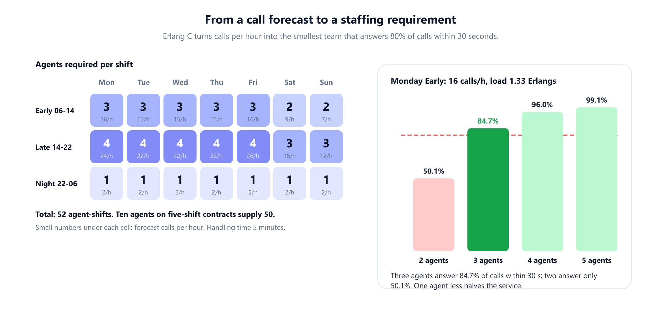
The numbers are steeper than intuition suggests. On Monday morning the desk expects 16 calls per hour, a workload of 1.33 agents' worth of calls. Three agents answer 84.7% of calls within 30 seconds. Two agents, still more than the raw workload, answer only 50.1%. Queues are non-linear: the last agent on a small team buys far more service than the average agent. The same pattern holds on the busiest shift of the week, Friday Late, with 26 calls per hour, where four agents reach 81.9% and three reach 51.7%.
Applied to every shift, the forecast gives 3 Early, 4 Late and 1 Night agent on weekdays and 2 Early, 3 Late and 1 Night at the weekend. That is 52 agent-shifts in the week. Ten agents on five-shift contracts supply 50, so before any rostering decision is made, at least two shifts will have to be bought.
Two simplifications are worth stating. Real contact centres forecast in 15 or 30 minute intervals rather than whole shifts, and then choose shift start times and breaks to follow the curve, which is exactly the problem Edie and Dantzig were solving. And Erlang C ignores callers who hang up, so it tends to overstate the staff needed; the Erlang A model adds abandonment. Neither changes the rostering method that follows.
4. The rules as a graph: every legal week is a path
The desk runs three 8-hour shifts: Early from 06:00 to 14:00, Late from 14:00 to 22:00 and Night from 22:00 to 06:00. Three rules constrain who can work what.
- Rest between shifts. The European Working Time Directive (2003/88/EC) requires at least 11 consecutive hours of rest in every 24-hour period. That forbids three transitions from one day to the next: Late then Early leaves only 8 hours, Night then Early leaves none at all, and Night then Late leaves 8 hours.
- The contract. Each agent is contracted for five shifts a week. A sixth shift is allowed as overtime; a seventh is not.
- One shift per day. An agent works at most one of the three shifts on any day.
These rules have a natural picture. Draw seven columns, one per day, each with four nodes: Early, Late, Night and Off. Connect each node to every node in the next column, except along the three forbidden transitions. A legal working week for one agent is then a path from Monday to Sunday through this layered graph that visits at most six working nodes.
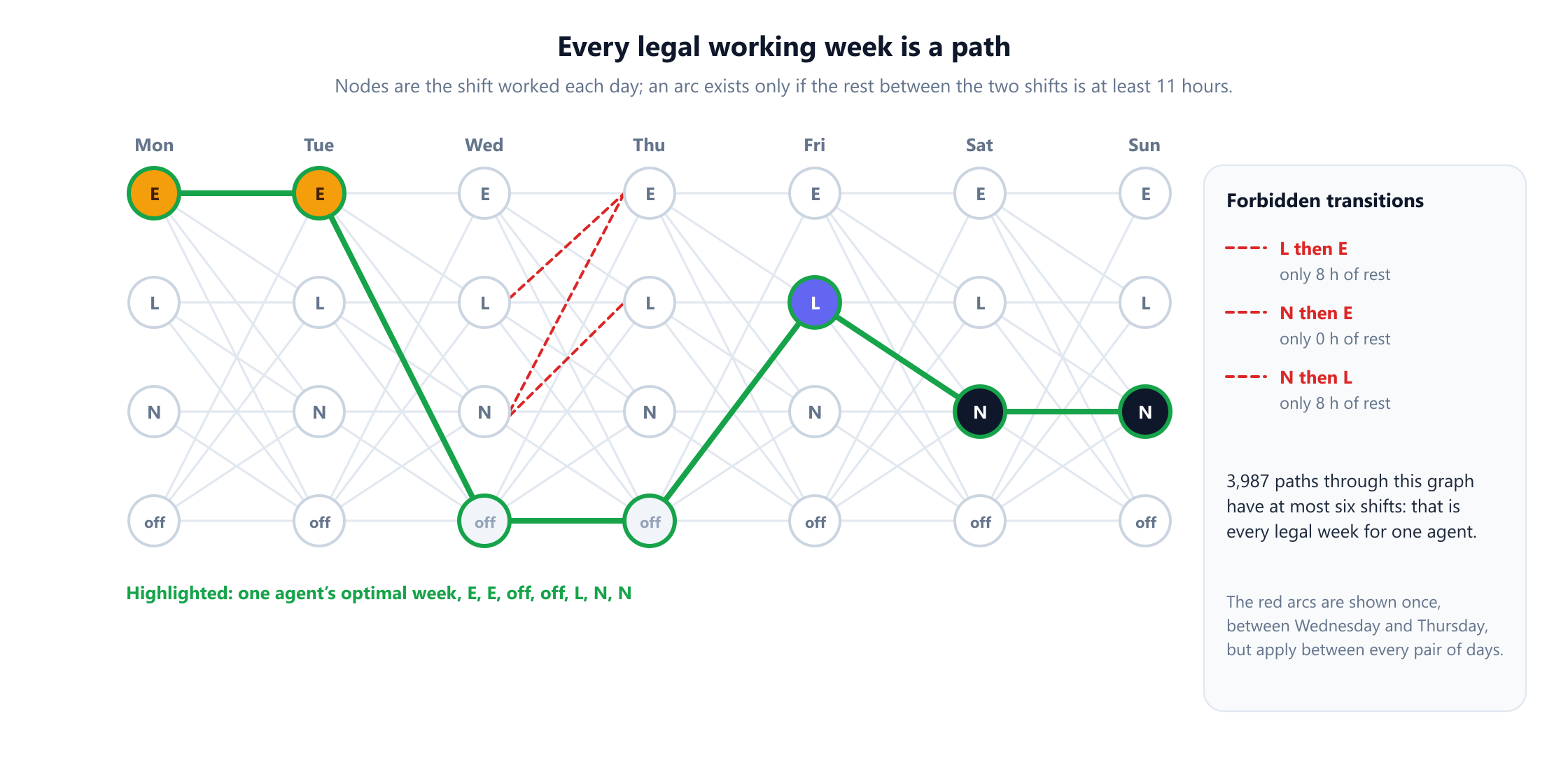
The graph makes the size of the problem concrete. There are 47 = 16,384 ways to fill a week with four choices a day. The three forbidden transitions and the six-shift limit leave 3,987 legal weeks for a single agent, assuming the agent was off the day before the week begins. Counting them does not require listing them: because the graph is acyclic, the number of paths into each node is the sum over its incoming arcs, one pass from Monday to Sunday, the same dynamic programming idea behind topological ordering.
A roster gives each of the ten agents one of those weeks, so there are 3,98710, about 1036, ways to roster ten named agents. Nobody searches that space by hand. What makes it tractable is structure, and the next sections show both the structure and the mistakes that ignoring it produces.
5. The week used throughout
The requirement from section 3, day by day:
| Shift | Mon | Tue | Wed | Thu | Fri | Sat | Sun |
|---|---|---|---|---|---|---|---|
| Early 06:00-14:00 | 3 | 3 | 3 | 3 | 3 | 2 | 2 |
| Late 14:00-22:00 | 4 | 4 | 4 | 4 | 4 | 3 | 3 |
| Night 22:00-06:00 | 1 | 1 | 1 | 1 | 1 | 1 | 1 |
The team is ten identical agents, A1 to A10, each able to work any shift. Every roster below is judged on one number: what it adds to the $9,600 of salaries, in overtime and agency cover. Section 12 relaxes the assumption that everyone can do everything.
6. How rosters get made without optimisation
Two common approaches make a fair baseline, because both are what a careful person does without software.
Fixed teams. Many managers split the staff into an early team, a late team and a night team in proportion to the weekday requirement, 3 to 4 to 1, which for ten agents gives four earlies, five lates and one night agent. Each agent keeps the same shift all week, and days off are staggered in pairs so that they spread around the week. It is simple, predictable and popular with staff.
On this week it leaves three shifts uncovered. The single night agent takes the weekend off, so Saturday and Sunday nights have nobody, and the staggered days off leave the late team one agent short on Monday, while Sunday Early has one agent more than it needs. Fixed teams have no mechanism for moving someone into a gap, so the three shifts go to the agency: $1,152 on top of salaries, with no overtime and no unused contracted shifts.
Greedy, day by day. The second approach fills the calendar in order. On each day it staffs the Night shift first, then Early, then Late, and gives each slot to the eligible agent who has worked the fewest shifts so far, using overtime only when nobody under contract can take the shift. It is the natural algorithm to code, and on this week it covers every single shift.
It is also the most expensive roster in this article: $1,440, all of it overtime. Greedy asked five agents to work a sixth shift, while two other agents finished the week with three contracted shifts unused between them. The cause is the night shift. Because nights are filled first and go to whoever has worked least, greedy handed them alternately to A1 (Monday, Wednesday, Friday, Sunday) and A9 (Tuesday, Thursday, Saturday). A night forbids an Early or Late shift the next day, so each of them spent the day after every night unable to take the day shifts that their colleagues were then paid overtime to cover. A1 worked four shifts and A9 three.
The lesson generalises. A roster that covers every shift is not a good roster by that fact alone. Greedy made each decision sensibly and in isolation, and the rest rule turned a fair-looking spread of nights into $864 of waste.
7. Local search: repairing a roster one change at a time
Instead of building a roster in one pass, local search starts from any roster and keeps making small changes that lower the cost, until no small change helps. Two changes are enough here:
- Change one agent's assignment on one day, to a different shift or to a day off.
- Swap two agents' assignments on the same day.
A change is accepted only if every rest rule and the six-shift limit still hold and the added cost falls.
Starting from the fixed teams, local search needs three changes. A2 moves from Sunday Early, where the team had a spare agent, to the uncovered Sunday night, which saves an agency shift and brings the cost to $768. A1 then takes Saturday night as a sixth, overtime shift, replacing the agency at $384 with overtime at $288: $672. Finally A2 takes the short Monday Late shift as a sixth shift: $576. No single change or swap improves on that.
Starting from the greedy roster the story is different. One swap between A2 and A9 on Monday lowers the cost to $1,152, and then local search stops, with four overtime shifts still paid and two contracted shifts still unused. Every single change from that roster either breaks a rest rule or costs more, even though a much cheaper roster exists. This is a local optimum: fixing the night pattern requires changing several agents' weeks at once, which no single move can do.
So local search is powerful, and it is also only as good as where it starts. The question it cannot answer is whether $576 is the best possible or just the best nearby. That needs the exact model.
8. The exact model: rostering as set covering
Dantzig's 1954 formulation turns the whole roster into one integer programme, and the graph from section 4 supplies its columns.
- Variables. For each of the 3,987 legal weeks, an integer: how many agents work that week. For each of the 21 shifts, an integer: how many agency workers cover it.
- Constraints. For each shift, agents working it plus agency workers must reach the requirement. And the number of agents across all weeks must equal ten.
- Objective. Minimise overtime, $288 for each week that contains six shifts, plus $384 for each agency shift.
That is 4,008 variables and 22 constraints. The model is solved the standard way: first as a linear programme, allowing fractional agents, with the simplex method, and then, if the answer is fractional, by branch and bound, Land and Doig's 1960 method, which splits on a fractional variable and solves the two halves. On this week the linear programme's optimum is already a whole-number roster costing $576, so no branching is needed, and the solve takes a fraction of a second.
The linear programme also delivers something a heuristic never can: a proof. Along with its answer it returns a price for each constraint, called the dual. Here the prices say that each required agent-shift is worth $288 and each agent on the team is worth minus $1,440. Those prices are a certificate, because two checks show no roster can do better:
- No legal week is worth more than it costs at these prices. A week with w shifts, up to five, has no overtime and a priced value of 288w - 1,440, which is at most zero. A week with six shifts costs $288 and is valued at 1,728 - 1,440 = 288, exactly its cost. An agency shift costs $384 against a value of $288.
- Adding up the prices over the requirement gives a lower bound on every roster: 52 × $288 - 10 × $1,440 = $576.
In this case the bound matches simple arithmetic: 52 shifts are needed, 50 are contracted, and the cheapest way to buy the other two is overtime. That is not always so. Section 11 adds one rule and the bound rises above the arithmetic, and the certificate still proves the new optimum.
9. Five rosters for the same week, priced
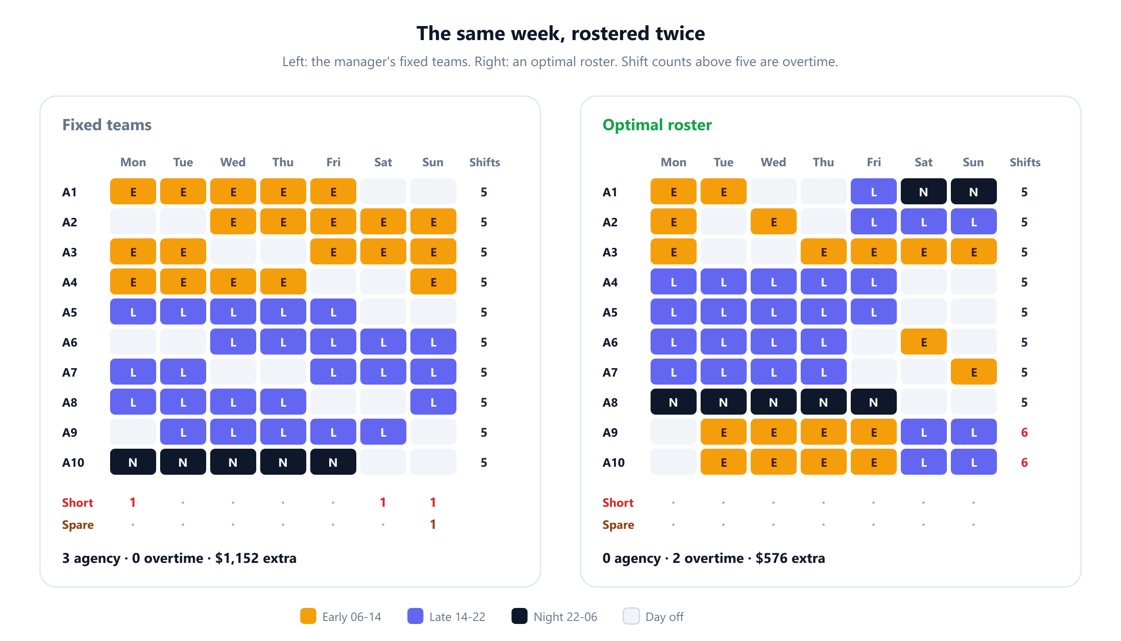
The optimum costs $576 on top of salaries: two overtime shifts, no agency and no unused contracted hours. Its structure is worth reading. A8 works the weeknight nights, Monday to Friday. A1 covers the weekend nights, working Early on Monday and Tuesday, then two days off, Late on Friday, and Night on Saturday and Sunday, a sequence in which no shift is followed by one the rest rule forbids. A9 and A10 each work the sixth shift. The optimum is not unique; the roster local search found from the fixed teams uses different weeks for the same cost.
| Method | Agency shifts | Overtime shifts | Unused contracted | Added cost | Above optimum |
|---|---|---|---|---|---|
| Fixed teams | 3 | 0 | 0 | $1,152 | +$576 |
| Greedy, day by day | 0 | 5 | 3 | $1,440 | +$864 |
| Greedy, then local search | 0 | 4 | 2 | $1,152 | +$576 |
| Fixed teams, then local search | 0 | 2 | 0 | $576 | 0 |
| Proven optimum | 0 | 2 | 0 | $576 | 0 |
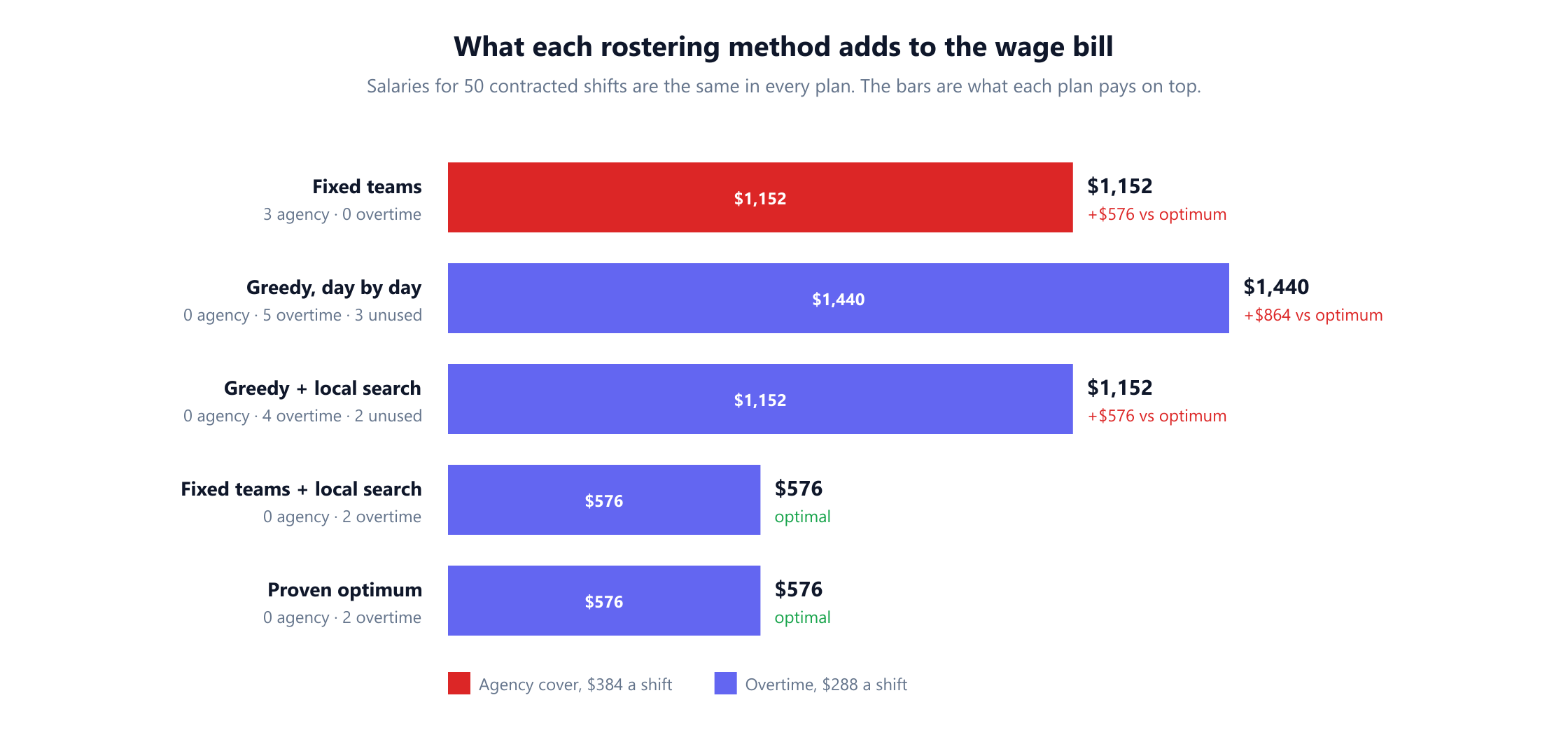
Three lessons stand out.
The desk was never short of people, only of good arrangements. The certificate proves that $576 is unavoidable with ten agents. Everything above it, $576 for the fixed teams and $864 for greedy, was waste created by the roster itself.
Full coverage is not efficiency. Greedy covered every shift and was the most expensive plan. Fixed teams left gaps and was cheaper. Coverage is a constraint; cost is the measure.
A good start matters to local search. The same moves turned one starting roster into an optimum and left the other stuck at double the optimal cost.
Over a year the gaps compound. If every week looked like this one, the fixed teams would cost about $30,000 more than the optimum over 52 weeks, and greedy about $45,000 more, for a team of ten.
10. Headcount: overtime or another hire?
The same model answers the question that sits above the roster: how many agents should the desk employ? Solving the week exactly for each team size, and adding salaries back in, gives the full weekly labour cost.
| Agents | Salaries | Overtime shifts | Agency shifts | Unused contracted | Total per week |
|---|---|---|---|---|---|
| 8 | $7,680 | 8 | 4 | 0 | $11,520 |
| 9 | $8,640 | 7 | 0 | 0 | $10,656 |
| 10 | $9,600 | 2 | 0 | 0 | $10,176 |
| 11 | $10,560 | 0 | 0 | 3 | $10,560 |
| 12 | $11,520 | 0 | 0 | 8 | $11,520 |
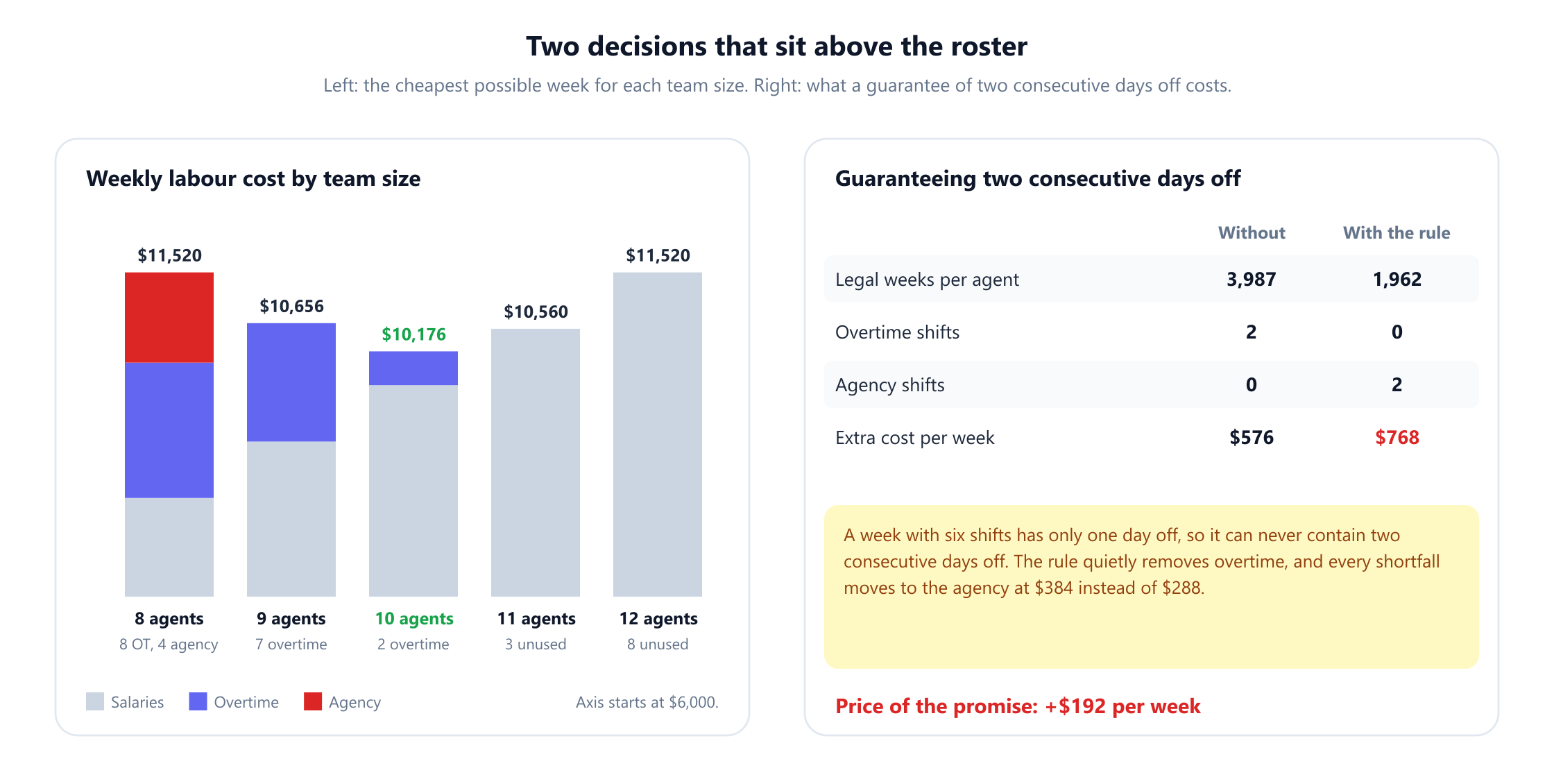
Ten agents is the cheapest team, at $10,176 a week. The reasoning on either side is instructive. Dropping to nine saves $960 of salary but needs five more overtime shifts, $1,440, so it costs $480 a week more. Adding an eleventh agent removes the $576 of overtime but adds $960 of salary, three shifts of which have nothing to do, so it costs $384 a week more.
The general rule behind the table: an extra hire pays for itself only if it removes more than a salary's worth of overtime and agency cost. At these prices a salary buys five shifts at $192 each, overtime costs $288 and agency $384, so a hire is worth it once the team would otherwise buy more than about three and a third overtime shifts a week, every week. A team that buys two, as here, should not hire.
One caution before acting on a table like this. It assumes everyone turns up. Real planning subtracts an allowance for holidays, sickness and training, usually called shrinkage, before sizing the team, and a team rostered to the exact minimum has no slack when someone calls in sick. The model handles that too, by solving with fewer available agents, but the allowance has to be a deliberate input.
11. Pricing a promise: two consecutive days off
Suppose the company wants to promise every agent two consecutive days off in each week, a common term in agreements with staff because split days off are tiring. It sounds almost free: every agent already has two days off in a five-shift week. The model says otherwise.
Adding the rule removes from the graph every week with no pair of adjacent days off between Monday and Sunday, and the number of legal weeks falls from 3,987 to 1,962. Re-solving gives a new optimum of $768, $192 a week more than before, about $10,000 over a year.
The mechanism is not obvious until the graph is examined. A week with six shifts has exactly one day off, so it can never contain two consecutive days off. The promise quietly abolishes overtime. The desk still needs two shifts beyond the 50 contracted, and with overtime gone, both have to come from the agency at $384 instead of $288. Two shifts at $96 more each is the $192.
This is also where the linear programme earns its keep. Simple arithmetic still says two extra shifts at the overtime price, $576. The linear programme, which knows that no six-shift week survives the rule, returns a bound of $768 straight away, and the whole-number roster meets it. Whether $192 a week is worth paying for better rest is a management decision; the model's job is to put the number on the table before the promise is made.
12. Skills: Hall's theorem on the night shift
Everything so far assumed that every agent can take every call. Real desks have skills: escalations that only senior staff handle, chat that only some agents are trained for. Skills turn "enough people on shift" into a different question, and graph theory answers it precisely.
Take one evening with five slots to fill: two escalation slots, one chat slot and two phone slots. Five agents are available: A1 handles phone and escalations, A2 phone, A3 phone and chat, A4 chat, and A5 phone. Five agents for five slots looks exactly right.
Draw agents on one side, slots on the other, and an edge wherever an agent holds the slot's skill. Filling the slots is finding a matching in this bipartite graph, a set of edges with no agent or slot used twice. The largest matching here covers only four of the five slots, and no rearrangement does better.
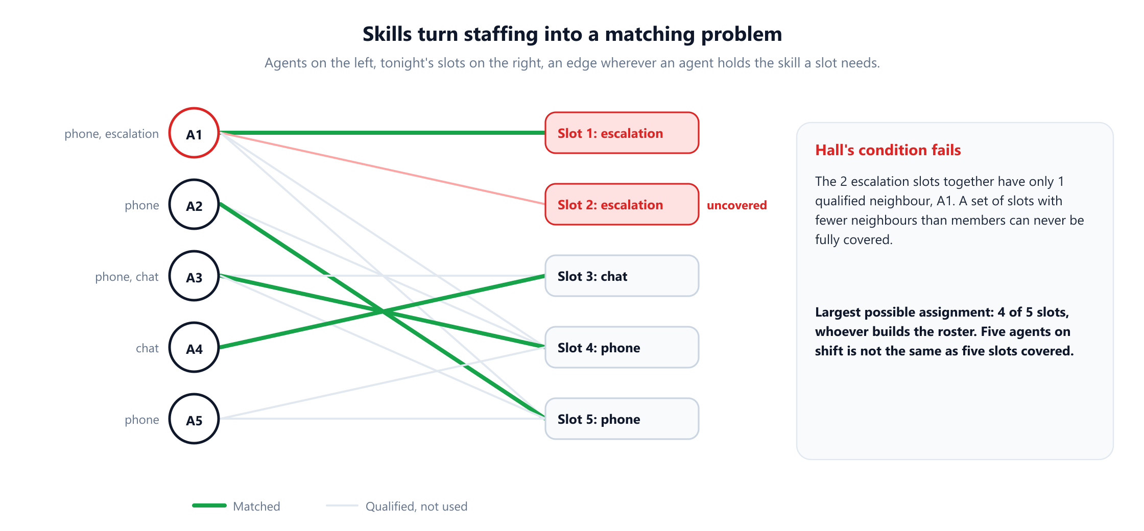
Hall's theorem (1935) explains why, and says what to look for. In a bipartite graph, every slot can be covered if and only if every set of slots has at least as many qualified agents as it has slots. Here the set of the two escalation slots has only one qualified agent, A1, so the condition fails. The theorem's deficiency form goes further: the largest matching covers all slots minus the worst shortfall over all sets, 5 - 1 = 4, which is exactly what the matching found.
Two practical points follow. The largest matching is computed in polynomial time, either with Kuhn's 1955 Hungarian method or as a maximum flow from a source through agents and slots to a sink, the construction Ford and Fulkerson made standard. And the violated set is diagnostic, not just a failure: it names the skill to train. One more escalation-trained agent fixes this evening, while training anyone for chat or phone changes nothing. When travel times, fairness and personal preferences enter the picture, the same matching becomes a full assignment problem, covered in our guide to assigning work fairly and cheaply.
In a full roster the same structure appears inside every shift. Skills enter the set covering model by grouping agents with the same skills, giving each group its own variables for its legal weeks, and requiring coverage separately for each skill. The model grows, but the logic, and Hall's warning that headcount can hide a skill gap, stays the same.
13. What is easy, what is hard
Knowing which parts of a rostering problem are easy is valuable, because it tells you where an answer can be exact and where it will be a good estimate.
| Question | Graph or model view | Difficulty |
|---|---|---|
| How many legal weeks does one agent have? | Counting paths in an acyclic layered graph | One pass, linear in the graph |
| Can tonight's slots be filled with these skills? | Bipartite matching, Hall's theorem | Polynomial |
| Fewest staff to cover fixed shift times on one day | Colouring an interval graph | Polynomial: the maximum number of shifts overlapping at one moment |
| Cyclic days-off patterns with consecutive days off | Integer programme with circular ones | Solvable through network flow structure (Bartholdi, Orlin and Ratliff, 1980) |
| A full roster with rest rules, contracts, skills and preferences | Set covering with side constraints | NP-hard in general |
The third row deserves a sentence of explanation. On a single day, shifts with fixed start and end times form an interval graph, where two shifts are adjacent if they overlap, and assigning workers so that nobody holds two overlapping shifts is colouring that graph. Interval graphs are perfect, so the minimum number of workers equals the largest set of shifts that all overlap at some moment, and a greedy sweep by start time achieves it.
The last row is the one that matters most in practice. Brucker, Qu and Burke's 2011 survey classifies the complexity of personnel scheduling models and shows that many practical variants are NP-hard. That does not mean real rosters are unsolvable, as this article's instance shows. It means the good methods are the ones that combine strong bounds with smart search: integer programming solvers, constraint programming, and metaheuristics tuned on benchmarks such as the International Nurse Rostering Competition of 2010.
14. What the model leaves out
The week above is a clean model. Real deployments add features that each have a well-studied extension.
- Intraday demand, start times and breaks. Requirements vary by the half hour, shifts can start at many times, and breaks must fall within windows. Bechtold and Jacobs (1990) and Aykin (1996) showed how to model flexible breaks without listing every combination.
- Preferences and fairness. Weekend work, nights and requested days off must be shared fairly over time. These usually enter as soft constraints with penalties, and the penalty weights are a management choice.
- Different contracts and wages. Part-time staff, different pay grades and minimum hours per contract change the cost of each week by person, so identical-agent models give way to one set of weeks per contract type.
- More legal limits. The same Directive also requires a weekly rest period and limits average weekly working time to 48 hours, and national law and collective agreements add their own rules.
- Longer horizons. This model assumes the previous day was off and ignores the following week. Real rosters run over four or more weeks, often as cyclic patterns that repeat, which Baker's 1974 survey reviews.
- Uncertain demand and absence. Forecasts are wrong and people are sick. Rosters are made robust with slack, flexible contracts and re-rostering closer to the day.
None of these changes the core picture: legal weeks as paths, coverage as constraints, and an optimiser with a bound. For the related problem of scheduling project work when people are the limiting resource, see graph theory in project management, and for scheduling drivers within vehicle routes, delivery route optimization.
15. Running a rostering project
The mathematics is the dependable part. Projects succeed or fail on four other things.
Get the requirement right. A roster optimised against a poor forecast is precisely wrong. Check the forecast against recent weeks, use realistic handling times, and agree the service target with the business before optimising anything.
Write down every rule, including the unwritten ones. Contracts, legal limits and agreements are the easy part. The rules that break rosters in practice are the informal ones: who never works with whom, who needs Tuesdays for a course. Collect them before the first roster, or the first roster will be rejected.
Price the current roster first. Cost last month's actual rosters with the same model. Without that baseline there is no way to show what optimisation earned, and the comparisons in section 9 are only meaningful because every roster was priced the same way.
Choose tools that fit, and involve the people rostered. Google OR-Tools includes a constraint programming solver, CP-SAT, that is widely used for shift scheduling; mixed integer programming solvers such as HiGHS, Gurobi and CPLEX solve set covering models directly; and commercial workforce management platforms add forecasting, shift swapping and self-service. Kellogg and Walczak's 2007 study of nurse scheduling found that few of the nurse scheduling models published in the research literature had been implemented in practice, a reminder that adoption, trust and the ability to swap shifts matter as much as the optimum.
16. Mistakes that quietly cost money
- Judging a roster by coverage alone. The greedy roster covered every shift and was the most expensive plan in section 9. Price overtime, agency and unused hours.
- Paying overtime while contracted hours go unused. Greedy paid five overtime shifts while two agents had three contracted shifts left between them. Look for both in the same week.
- Sizing the team from average workload. Two agents were more than Monday morning's workload and still answered only half the calls on time. Use a queueing model for the requirement.
- Treating headcount as the answer to every gap. An eleventh agent cost more than the overtime it removed. Price the hire against the overtime and agency it replaces.
- Making promises without pricing them. Two consecutive days off removed overtime altogether and added $192 a week. Re-solve before agreeing.
- Counting people instead of skills. Five agents could cover only four of five slots. Check Hall's condition for each skill-heavy shift.
- Ignoring the week boundary. A Sunday night followed by a Monday Early breaks the rest rule across weeks. Roster over a rolling horizon, or carry the previous week's last shift into the next.
- Trusting local search without a bound. From the greedy start, local search stopped at twice the optimal added cost. The linear programme's bound tells you how far from optimal a roster can be.
17. Frequently asked questions
What is employee shift scheduling?
+
It is the process of deciding which employees work which shifts over a planning period so that the required number of people, with the required skills, are present at each time, every legal and contractual rule is respected, and labour cost is as low as possible. In operations research it is also called personnel scheduling or rostering, and it is usually split into determining the staffing requirement, designing shifts, and assigning people to them.
How is a roster modelled as an optimization problem?
+
The classic model, due to Dantzig in 1954, is set covering. List every legal working pattern, for example every week a single employee may work under the rest rules and contract, and create an integer variable for how many people work each pattern. Add one constraint per shift requiring enough people, plus variables for overtime or agency cover, and minimise cost. The model is solved as a linear programme and then by branch and bound or with a constraint programming solver.
How do I calculate how many staff each shift needs?
+
For work that arrives randomly, such as calls, use a queueing model rather than dividing workload by productivity. Erlang C takes the arrival rate, the average handling time and a service target, such as 80% of calls answered within 30 seconds, and gives the smallest number of agents that meets it. In the example in this article, 16 calls per hour needed three agents: two agents, although more than the raw workload, would have answered only about half the calls on time.
Is it cheaper to hire another employee or pay overtime?
+
It depends on how much overtime and agency cover the extra person would actually remove, which a roster model can compute. In this article's example, a team of ten needed two overtime shifts a week; an eleventh agent would have removed $576 of overtime but added $960 of salary, so the week cost $384 more. A hire pays off only when it replaces more than a salary's worth of overtime and agency cost week after week, after allowing for absence.
Why is staff rostering so hard to solve?
+
Because the number of possible rosters is astronomical and the rules interact. In the example, a single agent has 3,987 legal weeks, so ten named agents can be rostered in about 10 to the power 36 ways, and a choice for one person changes what everyone else can do. Many practical variants are NP-hard. Real instances are still solved well by combining linear programming bounds with branch and bound, constraint programming or metaheuristics.
What does Hall's theorem have to do with scheduling?
+
Assigning qualified people to slots is a matching problem in a bipartite graph. Hall's theorem says every slot can be filled if and only if every set of slots has at least as many qualified people as slots. When it fails, the offending set names the missing skill. In the example, two escalation slots shared one qualified agent, so five agents could cover only four of five slots, and training one more person in escalations would fix it.
What software is used for staff scheduling optimization?
+
Google OR-Tools provides the CP-SAT constraint programming solver, which is widely used for shift scheduling, and mixed integer programming solvers such as HiGHS, Gurobi and CPLEX solve set covering formulations directly. Commercial workforce management platforms add forecasting, employee self-service and shift swapping on top of an optimiser. The right choice depends on the size of the workforce, how complex the rules are, and how rosters are published and changed.
18. References
The foundational papers, surveys and legal text behind the methods in this article, in chronological order.
- Erlang, A. K. (1917). “Solution of some problems in the theory of probabilities of significance in automatic telephone exchanges.” Elektroteknikeren, 13, 5–13 (in Danish).
- Hall, P. (1935). “On representatives of subsets.” Journal of the London Mathematical Society, 10(1), 26–30.
- Edie, L. C. (1954). “Traffic delays at toll booths.” Journal of the Operations Research Society of America, 2(2), 107–138.
- Dantzig, G. B. (1954). “A comment on Edie's ‘Traffic delays at toll booths’.” Journal of the Operations Research Society of America, 2(3), 339–341.
- Kuhn, H. W. (1955). “The Hungarian method for the assignment problem.” Naval Research Logistics Quarterly, 2(1–2), 83–97.
- Ford, L. R. and Fulkerson, D. R. (1956). “Maximal flow through a network.” Canadian Journal of Mathematics, 8, 399–404.
- Land, A. H. and Doig, A. G. (1960). “An automatic method of solving discrete programming problems.” Econometrica, 28(3), 497–520.
- Baker, K. R. (1974). “Workforce allocation in cyclical scheduling problems: a survey.” Operational Research Quarterly, 25(1), 65–76.
- Bartholdi, J. J., Orlin, J. B. and Ratliff, H. D. (1980). “Cyclic scheduling via integer programs with circular ones.” Operations Research, 28(5), 1074–1085.
- Bechtold, S. E. and Jacobs, L. W. (1990). “Implicit modeling of flexible break assignments in optimal shift scheduling.” Management Science, 36(11), 1339–1351.
- Aykin, T. (1996). “Optimal shift scheduling with multiple break windows.” Management Science, 42(4), 591–602.
- Gans, N., Koole, G. and Mandelbaum, A. (2003). “Telephone call centers: tutorial, review, and research prospects.” Manufacturing & Service Operations Management, 5(2), 79–141.
- European Parliament and Council (2003). “Directive 2003/88/EC concerning certain aspects of the organisation of working time.” Official Journal of the European Union, L 299, 9–19.
- Ernst, A. T., Jiang, H., Krishnamoorthy, M. and Sier, D. (2004). “Staff scheduling and rostering: a review of applications, methods and models.” European Journal of Operational Research, 153(1), 3–27.
- Burke, E. K., De Causmaecker, P., Vanden Berghe, G. and Van Landeghem, H. (2004). “The state of the art of nurse rostering.” Journal of Scheduling, 7(6), 441–499.
- Kellogg, D. L. and Walczak, S. (2007). “Nurse scheduling: from academia to implementation or not?” Interfaces, 37(4), 355–369.
- Brucker, P., Qu, R. and Burke, E. (2011). “Personnel scheduling: models and complexity.” European Journal of Operational Research, 210(3), 467–473.
- Van den Bergh, J., Beliën, J., De Bruecker, P., Demeulemeester, E. and De Boeck, L. (2013). “Personnel scheduling: a literature review.” European Journal of Operational Research, 226(2), 367–385.
- Haspeslagh, S., De Causmaecker, P., Schaerf, A. and Stølevik, M. (2014). “The first international nurse rostering competition 2010.” Annals of Operations Research, 218(1), 221–236.