
Table of Contents
- 1. When the budget, not the ideas, is the limit
- 2. How a single project is valued
- 3. The fourteen projects used throughout
- 4. How budgets usually get allocated
- 5. The best portfolio, and why it funds a losing project
- 6. Choosing projects as a longest path
- 7. Which projects are worth doing at all: a minimum cut
- 8. What another million is worth
- 9. Two years of cash limits
- 10. What is easy, what is hard
- 11. What the model leaves out
- 12. From spreadsheet to portfolio decision
- 13. Mistakes that quietly cost money
- 14. Frequently asked questions
- 15. References
1. When the budget, not the ideas, is the limit
Every year, finance teams collect investment proposals from across the business: a new production line, a warehouse, a software upgrade, a solar installation. Most of them are good projects, with positive net present value and a sound business case. And every year the total asked for is larger than the capital budget. Deciding which projects to fund, when there is not enough money for all of them, is capital rationing, and it is one of the most consequential decisions a management team makes.
Finance textbooks give a clear rule when money is unlimited: accept every project with a positive net present value. With a fixed budget that rule no longer works, and the most common substitutes, ranking projects by profitability index, internal rate of return or payback, are known to be unreliable. James Lorie and Leonard Savage showed in 1955 that choosing projects under a budget is a genuine optimisation problem, and Martin Weingartner solved it with integer programming in 1963. In the language of combinatorics it is a knapsack problem, and when projects depend on each other it gains a graph structure that network flow algorithms can exploit.
This article takes one company's fourteen candidate projects and a $10 million budget, and compares the ranking rules finance teams actually use with the proven best portfolio. Every number was computed exactly by checking every possible portfolio, not estimated.
2. How a single project is valued
- Net present value (NPV) discounts all future cash flows to today at the company's cost of capital, here 10% a year, and subtracts the investment. It is the value a project adds to the company.
- Profitability index is NPV divided by the investment: value created per dollar spent. With a single budget and divisible projects it is exactly the right ranking, which is why it is taught for capital rationing.
- Internal rate of return (IRR) is the discount rate at which NPV would be zero. It ignores the size of a project, so a small project with a spectacular return can outrank a large one that creates far more value.
- Payback is how many years it takes for cumulative cash flow to turn positive. It ignores everything after that point.
John Graham and Campbell Harvey's 2001 survey of 392 chief financial officers found that about three quarters always or almost always use NPV and IRR, and more than half use payback. All three are sensible for judging one project. The trouble starts when a list of projects must fit within a fixed amount of money.
3. The fourteen projects used throughout
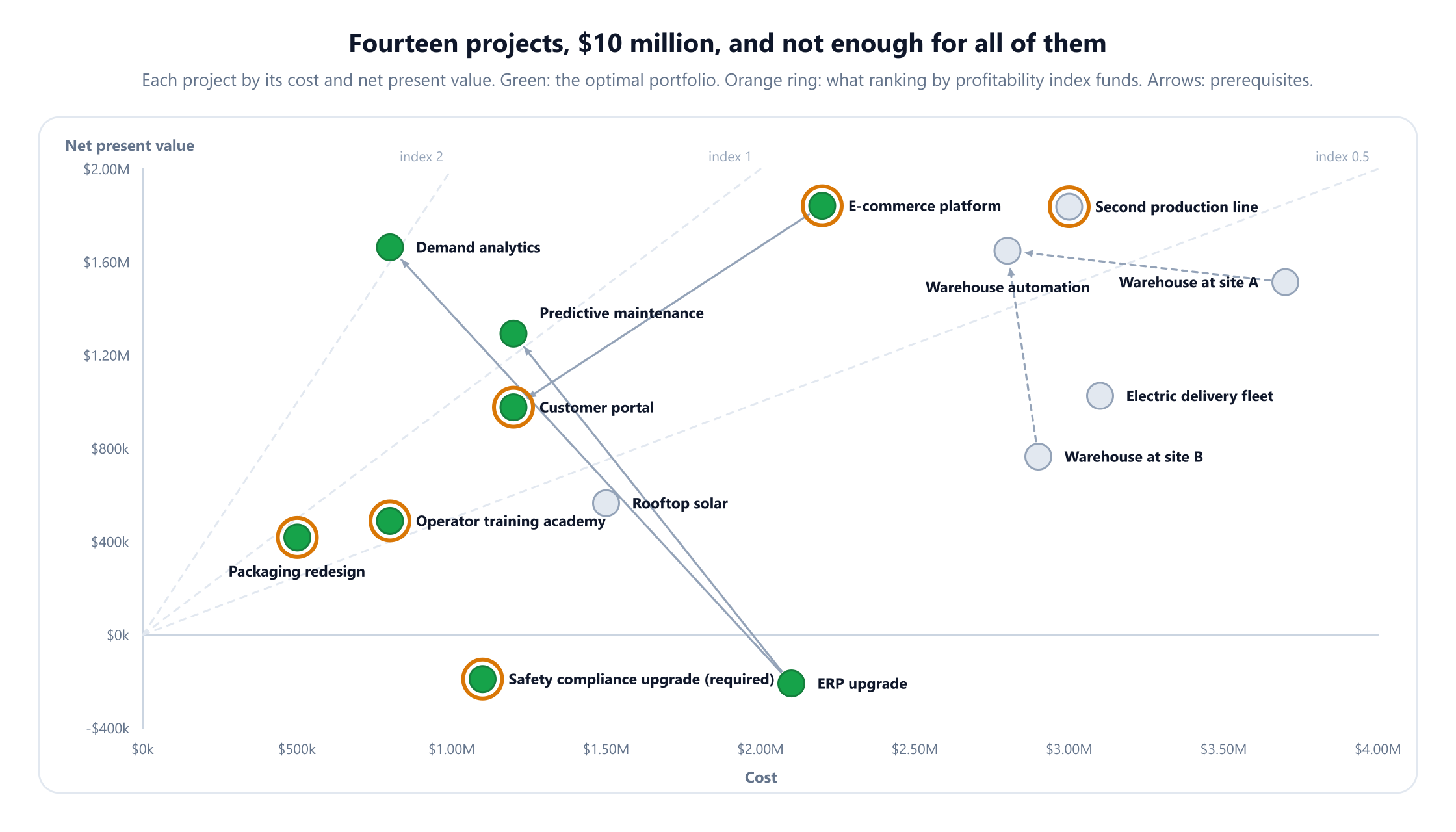
A mid-sized manufacturer has a capital budget of $10 million. Fourteen proposals have been submitted, with costs in thousands of dollars, a share of each cost that falls in the second year, a life over which the project brings a constant annual benefit, and the rules that link them:
| Project | Cost, $k | Spent next year | Life, years | Annual benefit, $k | NPV, $k | Profitability index | IRR | Payback, years | Condition |
|---|---|---|---|---|---|---|---|---|---|
| ERP upgrade | 2,100 | 25% | 10 | 300 | -209 | -0.10 | 7.5% | 7.0 | None |
| Demand analytics | 800 | 0% | 5 | 650 | 1,664 | 2.08 | 76.5% | 1.2 | Needs ERP upgrade |
| Predictive maintenance | 1,200 | 50% | 6 | 560 | 1,293 | 1.08 | 51.6% | 2.1 | Needs ERP upgrade |
| Warehouse at site A | 3,700 | 0% | 17 | 650 | 1,514 | 0.41 | 16.2% | 5.7 | Not with site B |
| Warehouse at site B | 2,900 | 25% | 16 | 460 | 765 | 0.26 | 14.5% | 6.3 | Not with site A |
| Warehouse automation | 2,800 | 50% | 8 | 810 | 1,649 | 0.59 | 28.0% | 3.5 | Needs a warehouse |
| Second production line | 3,000 | 50% | 12 | 690 | 1,838 | 0.61 | 23.4% | 4.3 | None |
| Rooftop solar | 1,500 | 50% | 25 | 220 | 565 | 0.38 | 15.3% | 6.8 | None |
| Packaging redesign | 500 | 50% | 3 | 360 | 418 | 0.84 | 74.2% | 1.4 | None |
| E-commerce platform | 2,200 | 25% | 7 | 820 | 1,842 | 0.84 | 35.0% | 2.7 | None |
| Customer portal | 1,200 | 50% | 5 | 560 | 977 | 0.81 | 47.8% | 2.1 | Needs e-commerce platform |
| Electric delivery fleet | 3,100 | 25% | 10 | 660 | 1,026 | 0.33 | 17.8% | 4.7 | None |
| Safety compliance upgrade | 1,100 | 50% | 10 | 140 | -190 | -0.17 | 5.2% | 7.9 | Required |
| Operator training academy | 800 | 0% | 5 | 340 | 489 | 0.61 | 31.8% | 2.4 | None |
Two projects lose money on their own. The ERP upgrade is an enabler: demand analytics and predictive maintenance cannot run without it. The safety compliance upgrade is required by regulation, whatever its return. The two warehouse sites are alternatives, and warehouse automation needs whichever is built. Together, all fourteen proposals ask for $26.9 million, and respecting their conditions leaves 2,400 possible portfolios. The figures are illustrative, but the structure, enablers, mandatory spending and alternatives, is what real capital budgets look like.
4. How budgets usually get allocated
The common approach is to sort the projects by a measure of attractiveness and fund them in that order until the money runs out, skipping any project that no longer fits. Every rule below funds the required safety upgrade first, never funds a project with negative NPV for its own sake, and skips a project whose prerequisite has not been funded when its turn comes.
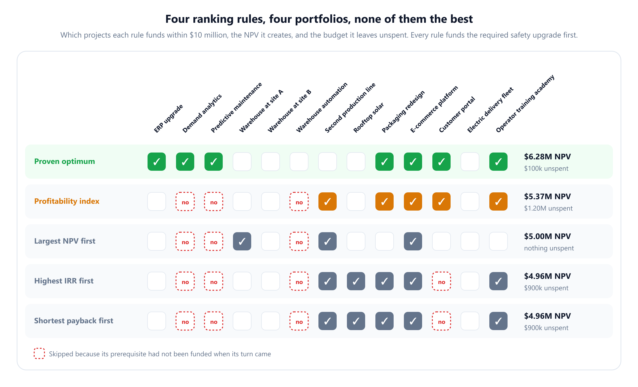
Largest NPV first. This rule funds the biggest value creators: the e-commerce platform, the second production line and the warehouse at site A. Demand analytics and predictive maintenance come up early but have no ERP system to run on. The rule spends every dollar and creates $5.00 million of NPV.
Profitability index. Demand analytics has by far the highest index, 2.08, but it is skipped at the top of the list because the ERP upgrade, with a negative index, is at the bottom. The rule then funds the e-commerce platform, packaging redesign, customer portal, second production line and training academy, and stops with $1.2 million unspent because nothing left fits. It creates $5.37 million.
Highest IRR first and shortest payback first reach the same portfolio here, because quick, high-return projects are the same projects. Both reach the customer portal before the e-commerce platform it needs, and both create $4.96 million.
5. The best portfolio, and why it funds a losing project
Checking every portfolio that respects the conditions and costs no more than $10 million finds the best one, and it is the only portfolio with that value. It funds the ERP upgrade, demand analytics, predictive maintenance, the e-commerce platform, the customer portal, packaging redesign, the training academy and the required safety upgrade, spends $9.9 million, and creates $6.28 million of NPV. The next best portfolio creates $5.87 million.
| Method | Spent | NPV created | Below the optimum |
|---|---|---|---|
| Highest IRR first | $9.1M | $4.96M | $1,322k (21.0%) |
| Shortest payback first | $9.1M | $4.96M | $1,322k (21.0%) |
| Largest NPV first | $10.0M | $5.00M | $1,280k (20.4%) |
| Profitability index | $8.8M | $5.37M | $910k (14.5%) |
| Proven optimum | $9.9M | $6.28M | 0 |
Two decisions explain the difference. The optimum pays $2.1 million for an ERP upgrade that loses $209,000 on its own, because it unlocks demand analytics and predictive maintenance, worth $2.96 million together for another $2.0 million. Judged as a package, the three projects create $2.75 million for $4.1 million, a profitability index of 0.67, which a project-by-project ranking can never see. And the optimum leaves out the second production line, the project with the second-largest NPV, because its $3 million buys more value elsewhere. Against the best ranking rule, the optimum creates $910,000 more from the same budget.
6. Choosing projects as a longest path
For independent projects, choosing a portfolio under a budget is the 0/1 knapsack problem: each project is in or out, costs add up to at most the budget, and values add up. Richard Bellman's dynamic programming solves it by building the portfolio one project at a time, and the calculation has a clean picture as a graph.
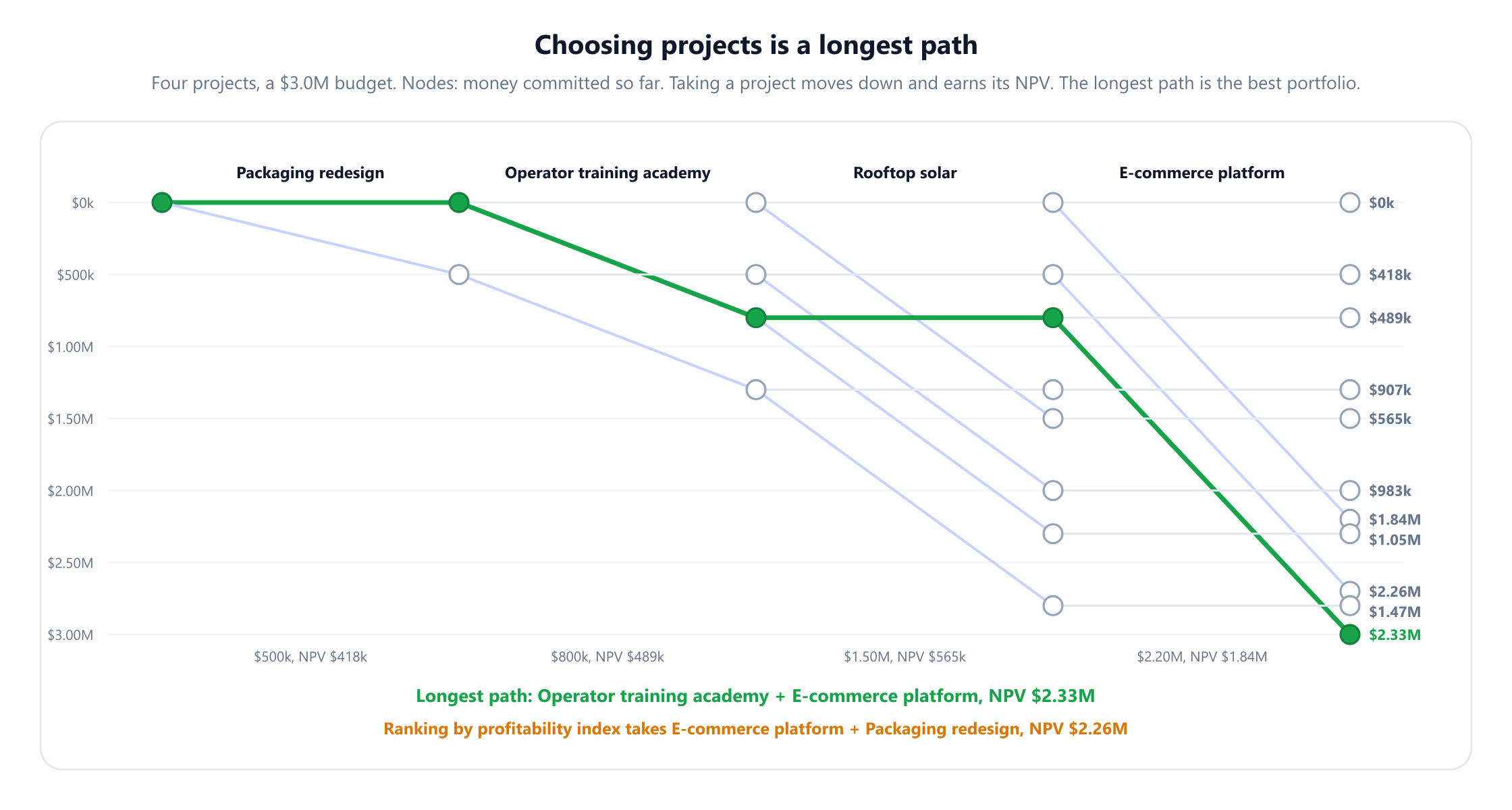
Take four independent projects and a $3.0 million budget. Draw a node for each amount of money committed after deciding on the first k projects. From each node, one edge skips the next project and one takes it, moving down by its cost and earning its NPV, provided the budget is not exceeded. Every portfolio is a path through this directed acyclic graph, and the best portfolio is the longest path, found in one pass from left to right. Here the graph has 26 nodes, and the longest path takes the training academy and the e-commerce platform for $2.33 million. Ranking by profitability index takes the e-commerce platform and packaging redesign, whose index is almost identical, for $2.26 million, leaving $300,000 of budget unused.
George Dantzig showed in 1957 that ranking by profitability index is exactly optimal if the last project can be funded partially. Real projects are rarely divisible, and that gap is why ranking fails. The knapsack problem is NP-hard, one of Richard Karp's 21 problems of 1972, but the dynamic programme and branch and bound solve realistic capital budgets, with hundreds of projects, in seconds. Kellerer, Pferschy and Pisinger's Knapsack Problems covers the methods in detail.
7. Which projects are worth doing at all: a minimum cut
Before asking what fits in the budget, it helps to ask which projects are worth doing if money were no object. With prerequisites, that is not simply "every project with positive NPV": an enabler with negative NPV is worth funding only if the projects it unlocks are worth more than it costs, and those projects may themselves unlock others.
A set of projects that includes every prerequisite of every project in it is called a closure of the prerequisite graph, and finding the most valuable closure is the maximum closure problem. J. M. W. Rhys and Michel Balinski showed in 1970, and Jean-Claude Picard proved in general in 1976, that it is solved by a minimum cut. Connect a source to every profitable project with capacity equal to its NPV, connect every loss-making project to a sink with capacity equal to its loss, and give every prerequisite link infinite capacity so it can never be cut. The projects on the source side of the minimum cut are the best closure.
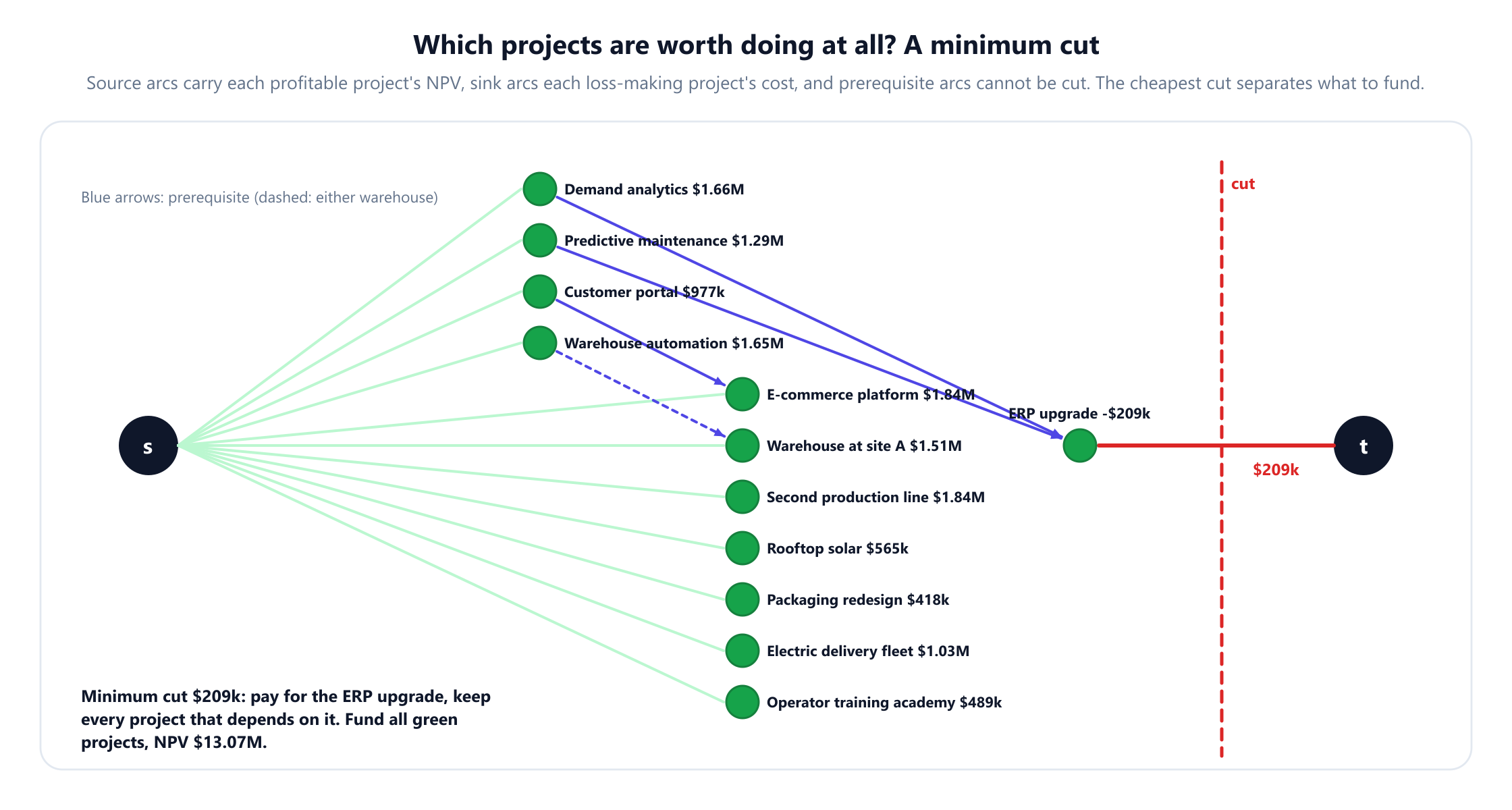
The warehouse alternatives break the closure structure, so the calculation is run once for each site. With site A, the profitable projects are worth $13.28 million in total, the minimum cut is $209,000, the ERP upgrade's loss, and the best closure is worth $13.07 million. With site B it is worth $12.32 million, so site A wins. Adding the required safety upgrade, everything worth doing costs $24.0 million and creates $12.88 million. Minimum cuts are computed in polynomial time, so this question can be answered exactly for thousands of interdependent projects, which Dorit Hochbaum's 2004 survey shows is how open-pit mine planning and many other selection problems are solved.
8. What another million is worth
Solving the portfolio for every budget, in steps of $100,000, shows what capital is worth at the margin.
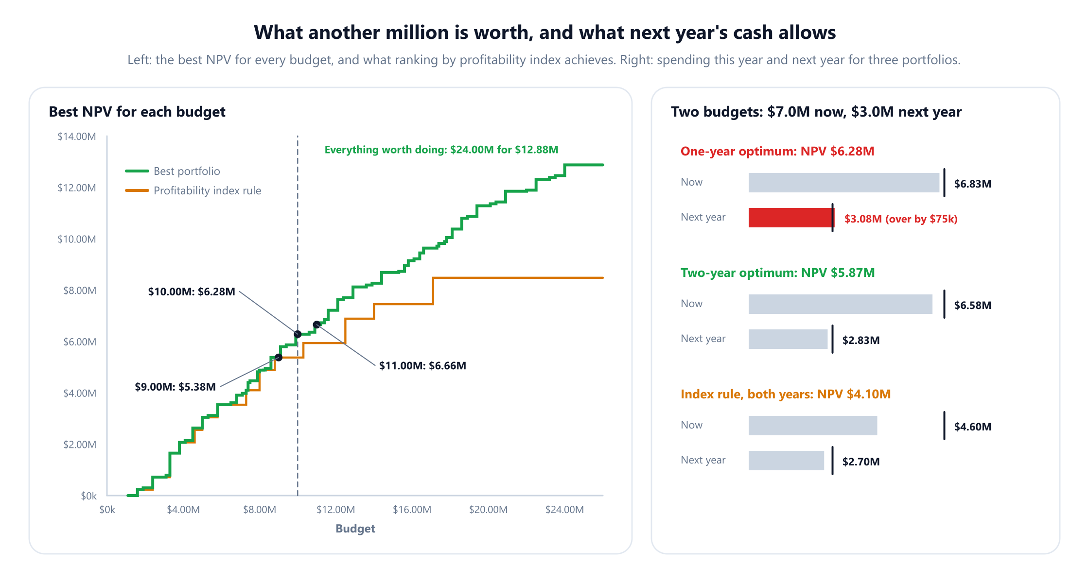
Raising the budget from $9 million to $10 million increases the best NPV from $5.38 million to $6.28 million, $907,000 of value for $1 million, because the extra money completes the ERP package. The next million adds only $372,000. Under the profitability index rule the same step from $9 million to $10 million adds nothing at all: the rule has no project that uses the extra million well. And with unlimited money the rule never goes above $8.48 million, because it never funds the ERP upgrade, while the best portfolio reaches $12.88 million.
These marginal values are the right input for the budget decision itself. If the company can borrow or reallocate a million dollars at a cost below the value it would create, the budget should rise; if not, it should not. A single fixed hurdle rate cannot capture that, because the value of capital depends on which projects are waiting at the margin.
9. Two years of cash limits
Many projects spend money over more than one year, and budgets are often set per year. Suppose the company can spend $7.0 million this year and $3.0 million next year. The one-year optimum spends $6.83 million this year, which fits, but $3.08 million next year, $75,000 over.
With a limit for each year the problem becomes a multidimensional knapsack, with one capacity per year. The best portfolio that respects both limits drops packaging redesign and creates $5.87 million. Losing $418,000 of value to save $75,000 of next year's cash is exactly the kind of trade-off that should be discussed rather than hidden: if the packaging project could be phased or if $75,000 could be found, the better portfolio is back. The profitability index rule, applied with both yearly limits, creates only $4.10 million, 30% less than the two-year optimum, because the second production line no longer fits next year and the rule has nothing good to replace it with.
Arnaud Fréville's 2004 survey explains why multiple budgets make the problem much harder: unlike the single knapsack, the multidimensional version has no efficient approximation scheme, as Magazine and Chern proved in 1984. In practice, integer programming solvers handle realistic multi-year capital budgets well.
10. What is easy, what is hard
| Problem | Method | Difficulty |
|---|---|---|
| Value of one project | Net present value | A formula |
| Divisible projects, one budget | Rank by profitability index (Dantzig, 1957) | Sorting |
| Whole projects, one budget | 0/1 knapsack: dynamic programming, branch and bound | NP-hard (Karp, 1972), pseudo-polynomial |
| Prerequisites, no budget | Maximum closure by minimum cut (Picard, 1976) | Polynomial |
| Prerequisites forming a tree, one budget | Tree knapsack dynamic programming (Johnson and Niemi, 1983) | Pseudo-polynomial |
| General prerequisites, one budget | Integer programming | NP-hard |
| Several yearly budgets | Multidimensional knapsack, integer programming | NP-hard, no efficient approximation scheme (Magazine and Chern, 1984) |
The practical reading is encouraging. Enumeration handles a few dozen projects, dynamic programming and integer programming handle hundreds with prerequisites, alternatives and several budgets, and minimum cuts handle the unbudgeted selection question at almost any size. Weingartner's 1966 survey of interrelated projects set out the integer programming formulations still used today.
11. What the model leaves out
- Risk. NPVs are estimates, and projects whose outcomes move together concentrate risk. Harry Markowitz's 1952 portfolio theory is the classic framework for balancing expected value against variance.
- Timing and flexibility. A project can often be delayed, phased or expanded later. Real options analysis, set out by Dixit and Pindyck in 1994, values that flexibility, and it can make waiting worth more than starting now.
- Strategic value. Some projects build capabilities or protect a market in ways that cash flow estimates capture poorly.
- Optimistic estimates. Proposals written to win funding tend to overstate benefits. Post-investment reviews of past projects are the best correction.
- Synergies and conflicts. Projects can make each other more or less valuable beyond simple prerequisites, which adds interaction terms to the model.
- A fixed budget. As section 8 showed, the budget itself is a decision, and the marginal value of capital should inform it.
12. From spreadsheet to portfolio decision
Standardise the proposals. Every proposal should state its cash flows by year, its dependencies on other proposals, its alternatives and whether it is required. Most of the value of optimisation comes from writing these links down, because ranking rules cannot use them.
Price the ranking you use today. Rebuild last year's funding decision with the same model and compare its NPV with the optimum. In the example, the best ranking rule left $910,000 of value unrealised from a $10 million budget.
Use an optimiser and show the trade-offs. A spreadsheet solver or an open-source mixed integer programming solver such as HiGHS handles the formulation directly. Present the best portfolio together with the value of more budget, the cost of each yearly limit and the next-best alternatives, so the investment committee debates trade-offs rather than rankings.
Keep judgment in the loop. Strategic and risk considerations belong in the decision. The model's role is to show exactly what each judgment costs, so that choosing a lower-value portfolio for a good reason is a deliberate choice rather than an accident of ranking. The facility location guide shows the same approach for choosing sites.
13. Mistakes that quietly cost money
- Ranking by IRR or payback. Both rules created $4.96 million, $1.32 million less than the optimum.
- Trusting the profitability index with whole projects. The best ranking rule still left $910,000 of value and $1.2 million of budget unused.
- Judging enablers on their own NPV. The ERP upgrade lost $209,000 alone but unlocked $2.96 million of value.
- Funding the biggest projects first. The optimum left out the project with the second-largest NPV.
- Treating the budget as fixed. The million dollars between $9 million and $10 million was worth $907,000; the next was worth $372,000.
- Ignoring next year's cash. The one-year best portfolio overspent next year by $75,000.
- Applying a ranking rule to yearly limits. It created 30% less value than the two-year optimum.
14. Frequently asked questions
What is capital rationing?
+
Capital rationing is the situation where a company has more projects with positive net present value than it can fund, because its capital budget is limited. The task is then to choose the combination of projects that creates the most value within the budget, taking into account prerequisites, alternatives, required projects and spending limits in each year.
Is the profitability index the right way to rank projects under a budget?
+
Only when projects can be funded partially and there is a single budget with no links between projects. With whole projects, prerequisites or several budgets it can be far from optimal. In the article's example, ranking fourteen projects by profitability index created $5.37 million of NPV, while the best portfolio within the same $10 million budget created $6.28 million.
Why not rank projects by IRR?
+
IRR measures the rate of return, not the amount of value created, so small projects with high returns outrank large projects that add more value, and it says nothing about how projects fit within a budget. In the example, ranking by IRR created $4.96 million of NPV, 21% less than the best portfolio.
How is capital budgeting related to the knapsack problem?
+
Choosing whole projects so that their total cost stays within a budget and their total value is as large as possible is exactly the 0/1 knapsack problem. It can be solved by dynamic programming, which is equivalent to finding a longest path in a layered graph of budget states, or by branch and bound and integer programming for larger portfolios with extra conditions.
Should a project with negative NPV ever be funded?
+
Yes, when it is required by regulation or when it enables other projects that are worth more than it costs. In the example an ERP upgrade lost $209,000 on its own but was needed by two projects worth $2.96 million, and the best portfolio funded it. Without a budget, deciding which enablers are worth funding is a maximum closure problem solved by a minimum cut.
How do you decide how large the capital budget should be?
+
Solve the portfolio for a range of budgets and look at how much value each additional amount of capital creates. Raise the budget while the value created by the next increment exceeds the cost of obtaining that capital. In the example, the million dollars between $9 million and $10 million created $907,000 of NPV, and the next million created $372,000.
What tools are used for capital budgeting optimization?
+
Small portfolios can be optimised with a spreadsheet solver. Larger ones with prerequisites, alternatives and several yearly budgets are formulated as mixed integer programs and solved with tools such as HiGHS, Gurobi or CPLEX, and project portfolio management software often includes such an optimiser. The inputs that matter most are consistent cash flow estimates and a clear record of how projects depend on each other.
15. References
The foundational papers, surveys and books behind the methods in this article, in chronological order.
- Markowitz, H. (1952). “Portfolio selection.” The Journal of Finance, 7(1), 77–91.
- Lorie, J. H. and Savage, L. J. (1955). “Three problems in rationing capital.” The Journal of Business, 28(4), 229–239.
- Bellman, R. (1957). Dynamic Programming. Princeton: Princeton University Press.
- Dantzig, G. B. (1957). “Discrete-variable extremum problems.” Operations Research, 5(2), 266–288.
- Weingartner, H. M. (1963). Mathematical Programming and the Analysis of Capital Budgeting Problems. Englewood Cliffs: Prentice-Hall.
- Weingartner, H. M. (1966). “Capital budgeting of interrelated projects: survey and synthesis.” Management Science, 12(7), 485–516.
- Balinski, M. L. (1970). “On a selection problem.” Management Science, 17(3), 230–231.
- Rhys, J. M. W. (1970). “A selection problem of shared fixed costs and network flows.” Management Science, 17(3), 200–207.
- Karp, R. M. (1972). “Reducibility among combinatorial problems.” In R. E. Miller and J. W. Thatcher (eds.), Complexity of Computer Computations, 85–103. New York: Plenum.
- Picard, J.-C. (1976). “Maximal closure of a graph and applications to combinatorial problems.” Management Science, 22(11), 1268–1272.
- Johnson, D. S. and Niemi, K. A. (1983). “On knapsacks, partitions, and a new dynamic programming technique for trees.” Mathematics of Operations Research, 8(1), 1–14.
- Magazine, M. J. and Chern, M.-S. (1984). “A note on approximation schemes for multidimensional knapsack problems.” Mathematics of Operations Research, 9(2), 244–247.
- Dixit, A. K. and Pindyck, R. S. (1994). Investment under Uncertainty. Princeton: Princeton University Press.
- Graham, J. R. and Harvey, C. R. (2001). “The theory and practice of corporate finance: evidence from the field.” Journal of Financial Economics, 60(2–3), 187–243.
- Fréville, A. (2004). “The multidimensional 0–1 knapsack problem: an overview.” European Journal of Operational Research, 155(1), 1–21.
- Hochbaum, D. S. (2004). “Selection, provisioning, shared fixed costs, maximum closure, and implications on algorithmic methods today.” Management Science, 50(6), 709–723.
- Kellerer, H., Pferschy, U. and Pisinger, D. (2004). Knapsack Problems. Berlin: Springer.
- Brealey, R. A., Myers, S. C. and Allen, F. (2020). Principles of Corporate Finance, 13th edition. New York: McGraw-Hill.