
Table of Contents
- 1. The short answer
- 2. One line of difference
- 3. One map, two searches
- 4. Why A* still finds the shortest path
- 5. The heuristic is a dial
- 6. How much A* saves on typical maps
- 7. The hidden cost of ties
- 8. When Dijkstra is the better choice
- 9. Heuristics that break the guarantee
- 10. Where each one is used
- 11. A short history
- 12. Common mistakes
- 13. Glossary
- 14. Frequently asked questions
- 15. References
1. The short answer
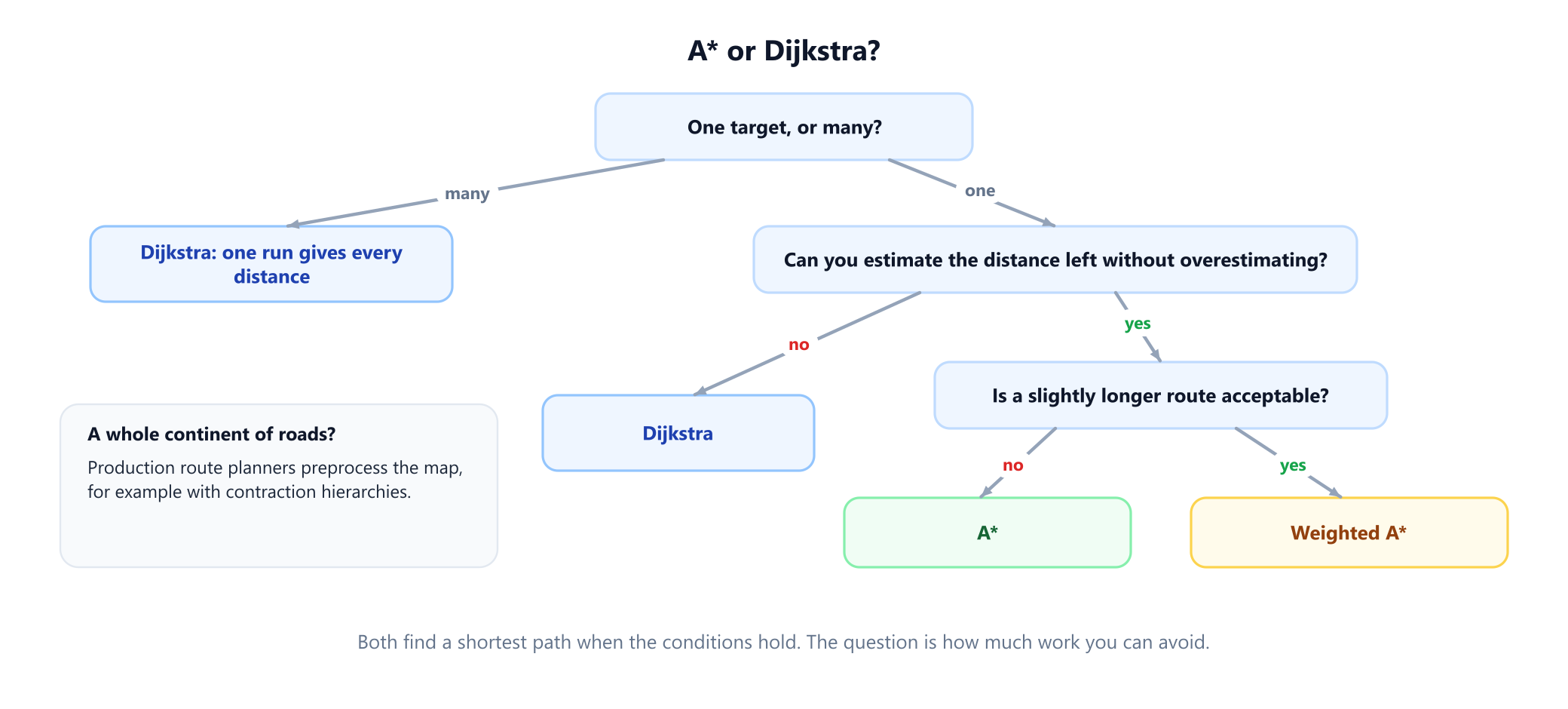
Dijkstra's algorithm and A* both find a shortest path in a weighted graph with nonnegative edge weights. The difference is what they know. Dijkstra searches outward in every direction, because it has no idea where the target is. A* adds an estimate of the remaining distance, so it spends its effort in the direction that looks promising.
| Dijkstra | A* | |
|---|---|---|
| Answers | One source to every vertex, or to one target | One source to one target |
| Priority of a vertex | g: distance from the source | f = g + h: distance so far plus estimated distance left |
| Needs | Nonnegative edge weights | Nonnegative edge weights and a heuristic h |
| Shortest path guaranteed | Yes | Yes, if h never overestimates |
| Vertices explored | Everything closer than the target | Usually far fewer; how many depends on h |
| Worst case on an explicit graph | O((V + E) log V) | The same, with a consistent h computed in constant time |
| Use it when | You need many targets or have no useful estimate | You want one route and can estimate the distance |
In one sentence: use A* for a single route on a map, where coordinates give you a good estimate, and use Dijkstra when you need distances to many places or when nothing tells you which way the target lies. The two are not rivals so much as the same algorithm with different information, as the next section shows. For how Dijkstra compares with methods that handle negative weights, see Dijkstra vs Bellman-Ford vs Floyd-Warshall.
2. One line of difference
Both algorithms keep a priority queue of vertices and repeatedly expand the one with the lowest priority. Write g(v) for the cost of the best route found so far from the start to v, and h(v) for an estimate of the cost from v to the goal, called the heuristic.
Dijkstra:   priority(v) = g(v)
A*:         priority(v) = g(v) + h(v)
That is the whole difference. Set h(v) = 0 for every vertex and A* becomes Dijkstra's algorithm. So every statement about Dijkstra is a statement about A* with the least informative heuristic possible, and everything A* gains comes from h. The guide to Dijkstra's algorithm and the guide to the A* search algorithm cover each one step by step.
The effect on the search is geometric. Dijkstra expands vertices in order of distance from the start, so its explored region grows like a circle. A* expands in order of the estimated total length of a route through each vertex, so vertices in the wrong direction get a high priority and are left in the queue. The circle becomes something closer to a narrow band from start to goal.
3. One map, two searches
The running example is a grid of 288 cells with a wall shaped like a cup, 24 cells of it blocked. A robot starts at S and has to reach G, moving one cell up, down, left or right at a cost of 1 per step. The wall forces a detour: on an empty grid G would be 22 steps away, but the shortest route takes 26. The heuristic is the Manhattan distance, the number of rows plus the number of columns between a cell and the goal, which ignores walls and so can never overestimate.
import heapq

MAP = ["........................",
       "..........#########.....",
       "..S...............#.....",
       "..................#.....",
       "..................#.....",
       "..................#..G..",
       "..................#.....",
       "..................#.....",
       "..................#.....",
       "..................#.....",
       "............#######.....",
       "........................"]

def locate(grid, ch):
    return next((r, row.index(ch)) for r, row in enumerate(grid) if ch in row)

def search(grid, start, goal, h, weight=1):
    """Best-first search on f = g + weight * h. With h = 0 this is Dijkstra."""
    g = {start: 0}
    done, count = set(), 0
    heap = [(weight * h(start), count, start)]
    while heap:
        _, _, u = heapq.heappop(heap)
        if u in done:
            continue                                   # stale entry
        done.add(u)
        if u == goal:
            return g[u], len(done)                     # path cost, vertices expanded
        r, c = u
        for v in ((r - 1, c), (r, c + 1), (r + 1, c), (r, c - 1)):
            if 0 <= v[0] < len(grid) and 0 <= v[1] < len(grid[0]) and grid[v[0]][v[1]] != '#':
                if g[u] + 1 < g.get(v, float('inf')):
                    g[v] = g[u] + 1
                    count += 1
                    heapq.heappush(heap, (g[v] + weight * h(v), count, v))
    return None

S, G = locate(MAP, 'S'), locate(MAP, 'G')
manhattan = lambda v: abs(v[0] - G[0]) + abs(v[1] - G[1])

print('Dijkstra        ', search(MAP, S, G, lambda v: 0))
# Dijkstra         (26, 232)
print('A* (Manhattan)  ', search(MAP, S, G, manhattan))
# A* (Manhattan)   (26, 149)
for w in (2, 5):
    print(f'weighted A*, w={w}', search(MAP, S, G, manhattan, weight=w))
# weighted A*, w=2 (26, 124)
# weighted A*, w=5 (26, 116)
print('greedy best-first', search(MAP, S, G, manhattan, weight=1000))
# greedy best-first (46, 108)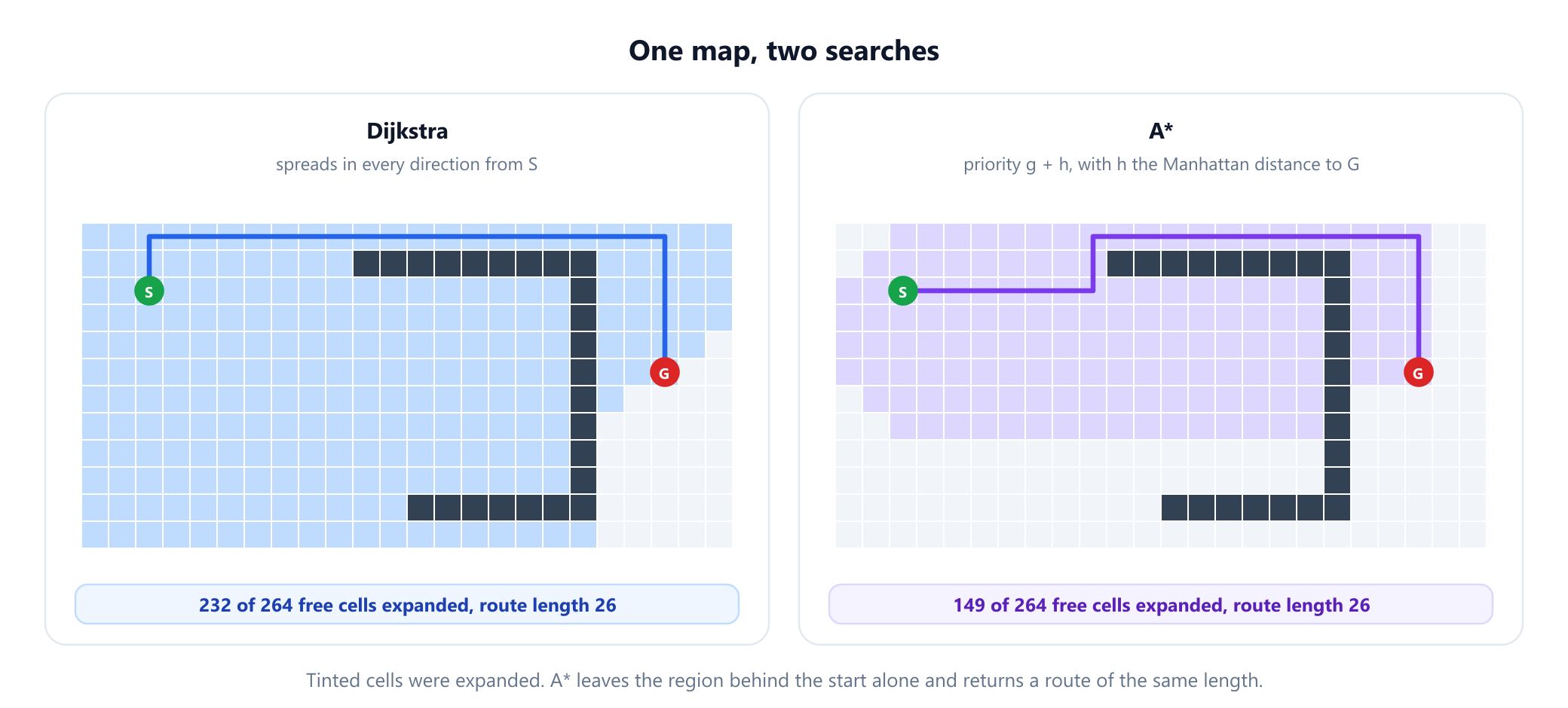
Both return a route of length 26. Dijkstra expands 232 of the 264 free cells before it reaches G, including cells on the far left that lead nowhere. A* expands 149. It does not need the full 232 because any cell whose f value exceeds 26 can never be on a shortest route, and A* never gets to them before it finishes.
That 36% saving is modest, because this map was built to fool the heuristic: inside the cup, the Manhattan distance keeps promising a straight run through the wall. Section 6 measures A* on 800 less hostile routes.
4. Why A* still finds the shortest path
An estimate sounds risky. The guarantee comes from one condition. A heuristic is admissible if it never overestimates the true remaining cost. Suppose A* is about to finish at the goal with a route of cost C, but a cheaper route of cost C* < C exists. Some vertex n on that cheaper route is still waiting in the queue, and because h never overestimates, f(n) = g(n) + h(n) ≤ C*. So f(n) is lower than the goal's priority C, and A* would have expanded n first. The cheaper route cannot be missed.
A stronger condition makes the implementation simple. A heuristic is consistent if, for every edge from u to v with weight w, h(u) ≤ w + h(v): moving one edge never lowers the estimate by more than that edge costs. With a consistent heuristic, A* never has to expand a vertex twice, exactly like Dijkstra. In fact, A* with a consistent heuristic is Dijkstra's algorithm run on the reweighted edges w'(u, v) = w(u, v) - h(u) + h(v), all of which are nonnegative. The guide to A* in AI gives the full proof and a counterexample for heuristics that are admissible but not consistent.
A* is also, in a precise sense, as economical as a one-directional safe search can be. Rina Dechter and Judea Pearl showed in 1985 that when the heuristic is consistent, any algorithm that expands vertices outward from the start, uses the same heuristic and is guaranteed to find a shortest path whenever the heuristic never overestimates must expand every vertex that A* is certain to expand, meaning every vertex that some path from the start reaches with f below the optimal cost. Only the handling of ties leaves room to do better, and two-way searches fall outside the result.
5. The heuristic is a dial
Between "knows nothing" and "knows everything" lies a whole range of behaviour, and the same code covers it, using a weight w in f = g + w * h. The output of the program in section 3 shows what happens on the example:
| Search | Priority | Cells expanded | Route length | Guarantee |
|---|---|---|---|---|
| Dijkstra | g | 232 | 26 | Shortest |
| A* | g + h | 149 | 26 | Shortest |
Weighted A*, w = 2 | g + 2h | 124 | 26 | At most 2 times the shortest |
Weighted A*, w = 5 | g + 5h | 116 | 26 | At most 5 times the shortest |
| Greedy best-first | h | 108 | 46 | None |
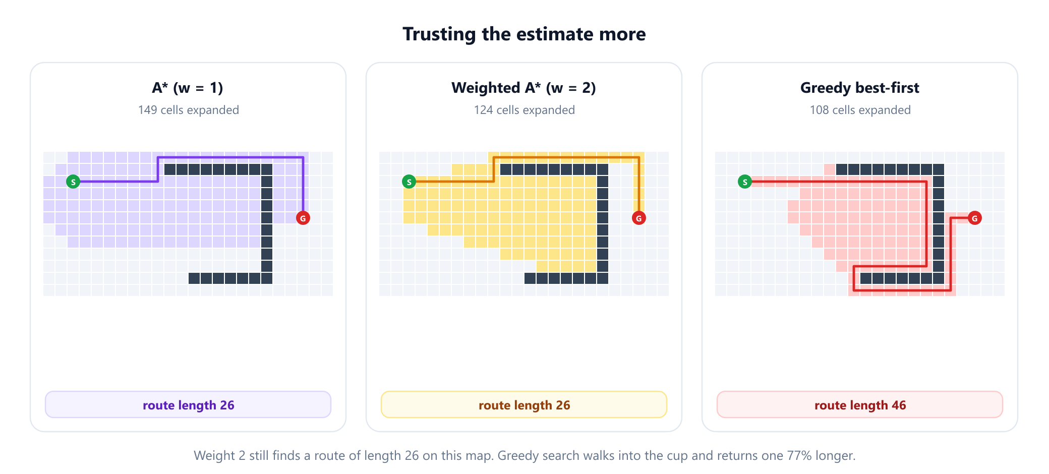
Weighted A* gives up the guarantee in a controlled way: with a consistent h, the route it returns is at most w times the shortest. On this map, weights of 2 and 5 still happen to find a route of length 26 with less work. Greedy best-first search, which ignores g altogether, saves only a little more and walks straight into the cup, returning a route of 46 steps, 77% longer than necessary. The work it saves is small compared with the quality it loses.
At the other end of the dial, a perfect heuristic, one that always equals the true remaining cost, would make A* walk almost directly to the goal. The closer an admissible h gets to the truth, the less A* expands. That is why heuristic design matters more than any implementation detail.
6. How much A* saves on typical maps
One map proves little. The program below compares the two searches over 200 random routes on each of four kinds of map: 60 by 60 grids with no walls, 20% walls and 35% walls, and a road network of 1,500 towns at random positions, each joined to its 4 nearest neighbours by a road up to 40% longer than the straight line. On the grids the heuristic is the Manhattan distance, and on the roads it is the straight-line distance. Dijkstra stops as soon as it reaches the target, which keeps the comparison fair.
import heapq, math, random

def search(neighbours, start, goal, h):
    """A*; pass h = lambda v: 0 for Dijkstra. Returns (cost, vertices expanded)."""
    g, done, count = {start: 0}, set(), 0
    heap = [(h(start), count, start)]
    while heap:
        _, _, u = heapq.heappop(heap)
        if u in done:
            continue
        done.add(u)
        if u == goal:
            return g[u], len(done)
        for v, w in neighbours(u):
            if g[u] + w < g.get(v, float('inf')):
                g[v] = g[u] + w
                count += 1
                heapq.heappush(heap, (g[v] + h(v), count, v))
    return None

def compare(neighbours, h_for, pairs):
    """Mean expansions of Dijkstra and of A* over the pairs that are connected."""
    dij = star = runs = 0
    for s, t in pairs:
        d = search(neighbours, s, t, lambda v: 0)
        if d is None:
            continue
        a = search(neighbours, s, t, h_for(t))
        assert abs(a[0] - d[0]) < 1e-9                 # same cost, every time
        dij += d[1]; star += a[1]; runs += 1
    return dij // runs, star // runs

def grid_trial(density, rnd, n=60, trials=200):
    wall = {(r, c) for r in range(n) for c in range(n) if rnd.random() < density}
    free = [(r, c) for r in range(n) for c in range(n) if (r, c) not in wall]
    def neighbours(u):
        r, c = u
        for v in ((r - 1, c), (r, c + 1), (r + 1, c), (r, c - 1)):
            if 0 <= v[0] < n and 0 <= v[1] < n and v not in wall:
                yield v, 1
    h_for = lambda t: lambda v: abs(v[0] - t[0]) + abs(v[1] - t[1])
    return compare(neighbours, h_for, [rnd.sample(free, 2) for _ in range(trials)])

def road_trial(rnd, n=1500, trials=200):
    """Towns at random points, each joined to its 4 nearest; roads wind up to 40% longer than the crow flies."""
    pts = [(rnd.random(), rnd.random()) for _ in range(n)]
    adj = [{} for _ in range(n)]
    for i, p in enumerate(pts):
        for j in sorted((j for j in range(n) if j != i), key=lambda j: math.dist(p, pts[j]))[:4]:
            w = math.dist(p, pts[j]) * rnd.uniform(1.0, 1.4)
            adj[i][j] = adj[j][i] = min(w, adj[i].get(j, w))
    neighbours = lambda u: adj[u].items()
    h_for = lambda t: lambda v: math.dist(pts[v], pts[t])
    return compare(neighbours, h_for, [rnd.sample(range(n), 2) for _ in range(trials)])

rnd = random.Random(1)
for density in (0.0, 0.2, 0.35):
    print(f'grid 60x60, {density:.0%} walls:', grid_trial(density, rnd))
print('road network, 1500 towns:', road_trial(rnd))
# grid 60x60, 0% walls: (1767, 451)
# grid 60x60, 20% walls: (1312, 238)
# grid 60x60, 35% walls: (1105, 397)
# road network, 1500 towns: (731, 235)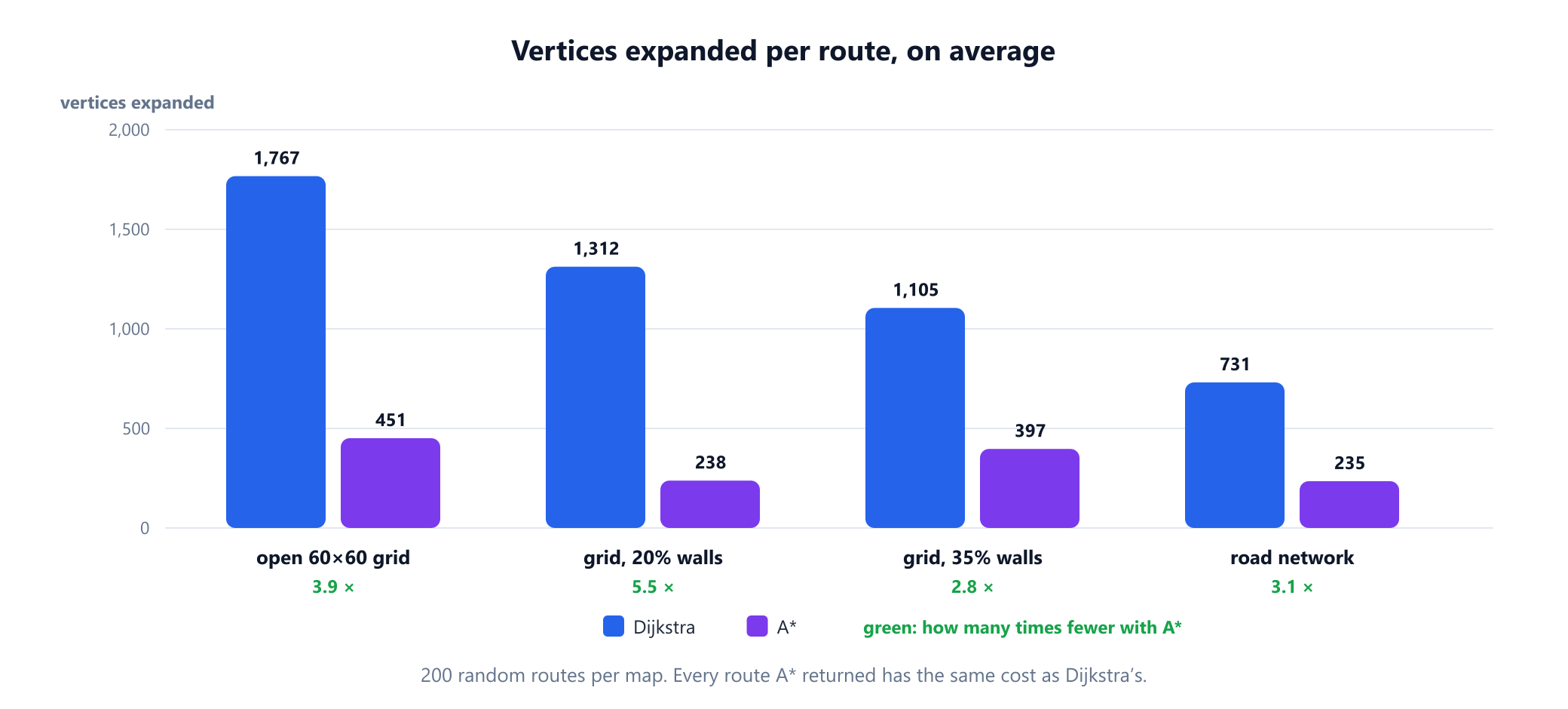
Across every map type, A* expanded about a third to a fifth of what Dijkstra did, and returned exactly the same cost on every route; the program checks that on each run. The saving is largest at 20% walls (about 5.5 times). On the empty grid it is smaller only because of the ties described in section 7, and at 35% walls (2.8 times) the frequent detours make the estimate less accurate. In the road network the saving is about 3 times, because roads wind and the straight-line distance is an underestimate.
Expanding fewer vertices does not automatically mean less time. A* has to compute h for every vertex it touches, and the priority queue holds more entries with similar priorities. On these maps the heuristic is one line of arithmetic, so the saving is real. A heuristic that is expensive to compute can give the advantage back.
7. The hidden cost of ties
On a grid with no walls, a huge number of cells have exactly the same f value, and the order in which A* takes them decides everything. The program below runs A* corner to corner across an empty 40 by 40 grid with three different tie-breaking rules.
import heapq

def expansions(n, tie):
    """A* across an empty n by n grid, corner to corner. tie(h, count) orders equal f values."""
    goal = (n - 1, n - 1)
    h = lambda v: abs(v[0] - goal[0]) + abs(v[1] - goal[1])
    g, done, count = {(0, 0): 0}, set(), 0
    heap = [(h((0, 0)), tie(h((0, 0)), 0), (0, 0))]
    while heap:
        _, _, u = heapq.heappop(heap)
        if u in done:
            continue
        done.add(u)
        if u == goal:
            return len(done)
        r, c = u
        for v in ((r - 1, c), (r, c + 1), (r + 1, c), (r, c - 1)):
            if 0 <= v[0] < n and 0 <= v[1] < n and g[u] + 1 < g.get(v, float('inf')):
                g[v] = g[u] + 1
                count += 1
                heapq.heappush(heap, (g[v] + h(v), tie(h(v), count), v))

n = 40
print('oldest entry first  ', expansions(n, lambda h, c: (c,)))
print('newest entry first  ', expansions(n, lambda h, c: (-c,)))
print('closest to the goal ', expansions(n, lambda h, c: (h, c)))
# oldest entry first   1600
# newest entry first   79
# closest to the goal  79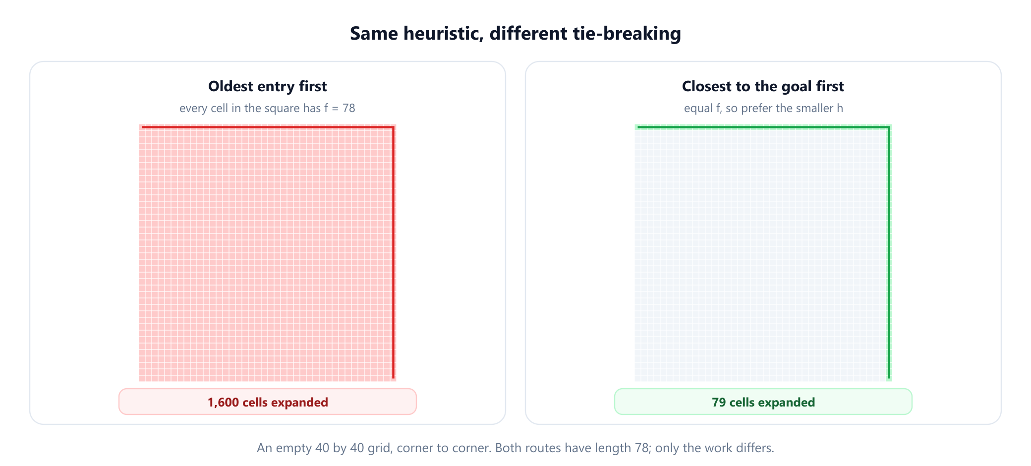
With ties broken in favour of the oldest entry, A* expands all 1,600 cells, no better than Dijkstra. Prefer the cell with the smaller h, which is the one with the larger g, and it expands 79, the cells of a single route; taking the newest entry first happens to do the same here. Every cell in the square lies on some shortest route, so all of them have f = 78; the rule simply decides whether to explore all those equally good routes or to commit to one. When comparing A* implementations, the tie-breaking rule can matter more than the data structure.
8. When Dijkstra is the better choice
- You need many targets. A single Dijkstra run from a source gives the distance to every vertex. Running A* once per target repeats work, and a heuristic aimed at one goal is useless for the others.
- There is no meaningful estimate. A* needs some notion of how far the goal is. In a social network, a citation graph or a dependency graph there are no coordinates to measure from, and
h = 0turns A* back into Dijkstra with extra bookkeeping. - The target is close to everything. If the goal is near the start or the graph is small, there is little to save.
- The answer is reused. A distance table or shortest-path tree computed once by Dijkstra can serve many later queries from the same source.
- You want the simplest correct code. Dijkstra has no heuristic to design or get wrong.
And some problems need neither. If every edge counts the same, breadth-first search finds shortest routes without any priority queue, as BFS vs DFS explains.
9. Heuristics that break the guarantee
A* is only as trustworthy as its heuristic, and the classic error is to use one that was designed for different moves. The Manhattan distance is safe when you can only move in four directions. Allow diagonal moves and it overestimates, since one diagonal step covers what it counts as two. The correct estimate for eight-way movement is the octile distance. The next program uses straight moves of cost 10 and diagonal moves of cost 14 on the same map.
import heapq

MAP = ["........................",
       "..........#########.....",
       "..S...............#.....",
       "..................#.....",
       "..................#.....",
       "..................#..G..",
       "..................#.....",
       "..................#.....",
       "..................#.....",
       "..................#.....",
       "............#######.....",
       "........................"]
STEPS = [(-1, 0, 10), (0, 1, 10), (1, 0, 10), (0, -1, 10), (-1, 1, 14), (1, 1, 14), (1, -1, 14), (-1, -1, 14)]

def search(start, goal, h):
    """A* with 8 directions: straight moves cost 10, diagonal moves 14."""
    g, done, count = {start: 0}, set(), 0
    heap = [(h(start), count, start)]
    while heap:
        _, _, u = heapq.heappop(heap)
        if u in done:
            continue
        done.add(u)
        if u == goal:
            return g[u], len(done)
        for dr, dc, w in STEPS:
            v = (u[0] + dr, u[1] + dc)
            if 0 <= v[0] < len(MAP) and 0 <= v[1] < len(MAP[0]) and MAP[v[0]][v[1]] != '#':
                if g[u] + w < g.get(v, float('inf')):
                    g[v] = g[u] + w
                    count += 1
                    heapq.heappush(heap, (g[v] + h(v), count, v))

S, G = (1, 19), (10, 0)                        # top right to bottom left, around the wall
def manhattan(v):
    return 10 * (abs(v[0] - G[0]) + abs(v[1] - G[1]))
def octile(v):
    dr, dc = abs(v[0] - G[0]), abs(v[1] - G[1])
    return 10 * max(dr, dc) + 4 * min(dr, dc)

print('Dijkstra ', search(S, G, lambda v: 0))
print('octile   ', search(S, G, octile))
print('Manhattan', search(S, G, manhattan))
# Dijkstra  (234, 261)
# octile    (234, 21)
# Manhattan (288, 45)
Dijkstra and A* with the octile distance both find the true shortest route, of cost 234, and A* needs only 21 expansions instead of 261. The Manhattan distance returns a route of cost 288, 23% too long, and gives no warning. An overestimating heuristic is fast and wrong at the same time, which makes it easy to miss.
Two related traps are worth knowing. A heuristic can be admissible yet inconsistent, in which case a vertex may need to be expanded more than once: an implementation with a closed set that refuses to reopen vertices, like the ones here, can then return a route that is not the shortest. And negative edge weights break both algorithms, for which see the Bellman-Ford algorithm.
10. Where each one is used
- Games. A* on grids and navigation meshes is the standard for unit movement. Jump Point Search, by Daniel Harabor and Alban Grastien, speeds up A* on uniform grids by skipping cells that symmetric routes make redundant.
- Robotics. A* was created for this: Peter Hart, Nils Nilsson and Bertram Raphael developed it at the Stanford Research Institute, and the IEEE Milestone for the Shakey robot credits that project with it.
- Networks. Link-state routing protocols such as OSPF use Dijkstra, since each router needs routes to every destination rather than one.
- Continent-scale road routing. Plain Dijkstra and plain A* are both too slow for a whole continent. The continent-scale systems that have been publicly documented preprocess the map. Contraction hierarchies add shortcut edges in advance, and ALT combines A* with distances to a few chosen landmarks to get a better heuristic.
- Puzzles and planning. A* and its memory-saving variant IDA*, due to Richard Korf, solve problems such as the sliding-tile puzzle, where the graph is far too large to store and is generated as the search runs.
Memory is often the real limit. Both algorithms store every vertex they have reached, so on huge implicit graphs A* can run out of memory long before it runs out of time. That is the case IDA* was built for.
11. A short history
Edsger Dijkstra published his algorithm in 1959. Nine years later, Hart, Nilsson and Raphael published A* in "A Formal Basis for the Heuristic Determination of Minimum Cost Paths", and in 1972 they published a short correction about the role of consistency in their optimality proof. Ira Pohl studied weighted evaluation functions in 1970. Dechter and Pearl set out in 1985 exactly in which sense A* is optimal. The two algorithms are often presented as a progression, but as section 2 showed, A* contains Dijkstra as the special case h = 0.
12. Common mistakes
| Mistake | Why it is wrong | Fix |
|---|---|---|
| Using A* to compute many targets | The heuristic points at one goal, and the work is repeated for each | Run Dijkstra once from the source |
| Using Manhattan distance with diagonal moves | It overestimates, and on the example returns 288 instead of 234 | Use the octile distance |
| Assuming A* is always faster | With h = 0 or a costly h it does the same work or more | Measure, and keep the heuristic cheap |
| Ignoring ties | On an open 40 by 40 grid the rule changes 1,600 expansions to 79 | Break ties toward the smaller h |
| Comparing against a Dijkstra that does not stop at the target | A full run explores the whole graph and exaggerates the saving | Stop Dijkstra when the target is expanded |
| Treating greedy best-first as a faster A* | It has no guarantee and returned 46 steps instead of 26 | Use weighted A* if you want a bounded trade-off |
| Using a closed set with an inconsistent heuristic | A better route to a closed vertex is thrown away | Use a consistent heuristic, or allow reopening |
| Running either on negative edges | Both assume costs never decrease along a route | Use Bellman-Ford or Johnson's algorithm |
13. Glossary
| Term | Meaning |
|---|---|
| g(v) | The cost of the best route found so far from the start to v |
| h(v) | The heuristic: an estimate of the cost from v to the goal |
| f(v) | g(v) + h(v), the estimated total cost of a route through v |
| Expansion | Taking a vertex from the queue and examining its neighbours |
| Admissible heuristic | One that never overestimates the true remaining cost |
| Consistent heuristic | One with h(u) ≤ w + h(v) for every edge |
| Manhattan distance | Rows plus columns between two cells; safe for four-way movement |
| Octile distance | The grid distance when diagonal moves are allowed |
| Weighted A* | A* with f = g + w * h, trading route quality for speed |
| Greedy best-first search | Search ordered by h alone, with no guarantee |
| Tie-breaking | The rule that orders vertices with equal f values |
| IDA* | A depth-first variant of A* that uses very little memory |
14. Frequently asked questions
What is the difference between A* and Dijkstra?
Dijkstra orders vertices by g, the distance from the start. A* orders them by f = g + h, where h is an estimate of the distance remaining to the goal. With h = 0 the two are the same algorithm. The estimate lets A* concentrate on the direction of the goal, so it usually explores far fewer vertices while still finding a shortest path.
Is A* always faster than Dijkstra?
Not always. A* usually expands far fewer vertices when a good estimate exists: about three to five and a half times fewer in the random maps measured here. With a heuristic of zero, a heuristic that is slow to compute or poor tie-breaking, it can do as much work as Dijkstra or more. A single Dijkstra run is also better when you need distances to many targets.
Does A* always find the shortest path?
Only if the heuristic is admissible, meaning that it never overestimates the true remaining cost. If it can overestimate, A* may return a longer route without any warning. An implementation that never reopens a vertex also needs the heuristic to be consistent, meaning that h(u) is at most w(u, v) + h(v) for every edge.
Is A* the same as Dijkstra with a heuristic?
Yes, in a precise sense. A* with h = 0 is Dijkstra's algorithm, and A* with a consistent heuristic behaves exactly like Dijkstra run on the reweighted edges w(u, v) - h(u) + h(v), all of which are nonnegative.
When should I use Dijkstra instead of A*?
Use Dijkstra when you need distances from one source to many or all vertices, when no useful estimate of the remaining distance exists, as in social or dependency graphs, or when the simplest correct code matters most. Use A* when you want one route to one target and can estimate the distance, for example from coordinates on a map.
What is the best heuristic for A* on a grid?
It depends on the moves. Use the Manhattan distance for four-way movement and the octile distance when diagonal moves are allowed. Using the Manhattan distance with diagonal moves overestimates and can return a route that is too long. Breaking ties in favour of the vertex closer to the goal also makes a large difference on open grids.
15. References
The algorithms, results and attributions above come from these sources, listed in chronological order.
- Dijkstra, E. W. (1959). "A Note on Two Problems in Connexion with Graphs." Numerische Mathematik 1, 269 to 271.
- Hart, P. E., Nilsson, N. J. and Raphael, B. (1968). "A Formal Basis for the Heuristic Determination of Minimum Cost Paths." IEEE Transactions on Systems Science and Cybernetics 4(2), 100 to 107.
- Pohl, I. (1970). "Heuristic Search Viewed as Path Finding in a Graph." Artificial Intelligence 1(3 to 4), 193 to 204.
- Hart, P. E., Nilsson, N. J. and Raphael, B. (1972). "Correction to 'A Formal Basis for the Heuristic Determination of Minimum Cost Paths'." SIGART Newsletter 37, 28 to 29.
- Pearl, J. (1984). Heuristics: Intelligent Search Strategies for Computer Problem Solving. Reading, MA: Addison-Wesley.
- Dechter, R. and Pearl, J. (1985). "Generalized Best-First Search Strategies and the Optimality of A*." Journal of the ACM 32(3), 505 to 536.
- Korf, R. E. (1985). "Depth-First Iterative-Deepening: An Optimal Admissible Tree Search." Artificial Intelligence 27(1), 97 to 109.
- Moy, J. (1998). "OSPF Version 2." RFC 2328. Internet Engineering Task Force.
- Goldberg, A. V. and Harrelson, C. (2005). "Computing the Shortest Path: A* Search Meets Graph Theory." In Proceedings of the 16th ACM-SIAM Symposium on Discrete Algorithms, 156 to 165.
- Geisberger, R., Sanders, P., Schultes, D. and Delling, D. (2008). "Contraction Hierarchies: Faster and Simpler Hierarchical Routing in Road Networks." In Experimental Algorithms, Lecture Notes in Computer Science 5038, 319 to 333.
- Thayer, J. T. and Ruml, W. (2008). "Faster than Weighted A*: An Optimistic Approach to Bounded Suboptimal Search." In Proceedings of the 18th International Conference on Automated Planning and Scheduling, 355 to 362.
- Harabor, D. and Grastien, A. (2011). "Online Graph Pruning for Pathfinding on Grid Maps." In Proceedings of the 25th AAAI Conference on Artificial Intelligence, 1114 to 1119.
- Bast, H., Delling, D., Goldberg, A., Müller-Hannemann, M., Pajor, T., Sanders, P., Wagner, D. and Werneck, R. F. (2016). "Route Planning in Transportation Networks." In Algorithm Engineering, Lecture Notes in Computer Science 9220, 19 to 80.
Race them on your own map
Draw a wall in the A* visualizer and watch how far the search spreads. Then run Dijkstra on the same graph and compare how many vertices each one visits.
Open the visualizer