
Table of Contents
- 1. What a strongly connected component is
- 2. Every digraph is a DAG of components
- 3. The example used throughout
- 4. The obvious method, and why it is slow
- 5. What depth-first search reveals
- 6. Kosaraju-Sharir: two passes
- 7. Tarjan's algorithm: one pass with low-links
- 8. Bugs that survive small tests
- 9. The path-based algorithm
- 10. Which algorithm to use
- 11. Working with the condensation
- 12. Where SCCs are used
- 13. Frequently asked questions
- 14. References
In an undirected graph, one search tells you everything about connectivity: whatever it reaches is connected to where it started, both ways. Directed graphs break this symmetry. A web page can link to a site that never links back, and a function can call another that never calls it. To say which parts of a directed graph really hang together, you need a stronger notion of connection and a cleverer algorithm to find it.
That notion is the strongly connected component. Three linear-time methods find all of them, each built on depth-first search and each hiding a small idea that is easy to get subtly wrong. This guide traces all three on one example, proves why they work, shows the bugs that pass casual testing, and ends with applications from 2-SAT to the structure of the web. Every trace, table and output below was produced by running the code.
If the words arc, in-degree or strongly connected are new, the article on directed and undirected graphs covers them first.
1. What a strongly connected component is
Let G = (V, A) be a directed graph with n vertices and m arcs. Say that u reaches v when there is a directed path from u to v. Every vertex reaches itself through the path of length zero.
Two vertices are strongly connected when each reaches the other. A strongly connected component is a maximal set of vertices in which every pair is strongly connected.
The word maximal matters. In a directed triangle A → B → C → A, the pair {A, B} is strongly connected, but it is not a component, because C can be added without breaking the property. The component is the whole triangle.
Mutual reachability is an equivalence relation: reflexive because each vertex reaches itself, symmetric by definition, and transitive because paths concatenate. So every digraph partitions into strongly connected components in exactly one way, and a vertex that lies on no directed cycle is a component on its own.
A digraph is strongly connected when it has a single component. It is weakly connected when it would be connected with arc directions ignored, and unilaterally connected when, for every pair, at least one reaches the other. Harary, Norman and Cartwright laid out this hierarchy in 1965: strong implies unilateral implies weak, and neither converse holds.
2. Every digraph is a DAG of components
Contract each strongly connected component to a single vertex, and keep an arc from component C to component D whenever some arc of G runs from a vertex of C to a vertex of D. The result is the condensation of G, sometimes called the component graph.
The condensation of any directed graph is a directed acyclic graph.
The proof takes one sentence. If the condensation contained a cycle through components C1, C2, ..., Ck, every vertex of every one of those components could reach every other by going around the cycle, so they would all be one component, contradicting maximality.
This is what makes SCCs so useful. Any directed graph, however tangled, is a DAG whose nodes happen to contain cycles: the cyclic behaviour is sealed inside components, and between components everything flows one way. Tools that need a DAG, such as topological sorting, longest paths and dynamic programming over dependencies, apply to any digraph once its components are contracted. And since a finite DAG has at least one source (no incoming arcs) and one sink (no outgoing arcs), every digraph has at least one source component and one sink component.
3. The example used throughout
All three algorithms below run on one digraph with nine vertices and twelve arcs. Neighbours are listed alphabetically, which fixes the order a depth-first search explores them:
A: B          D: E          G: H
B: C, F       E: C          H: D, G, I
C: D          F: A, G       I: (none)
Three of the mistakes in section 8 change the answer on it. It has four components: the directed triangle {A, B, F}, the directed triangle {C, D, E}, the two-cycle {G, H}, and the lone vertex {I}, which lies on no cycle. The arcs between components are B → C, F → G, H → D and H → I.
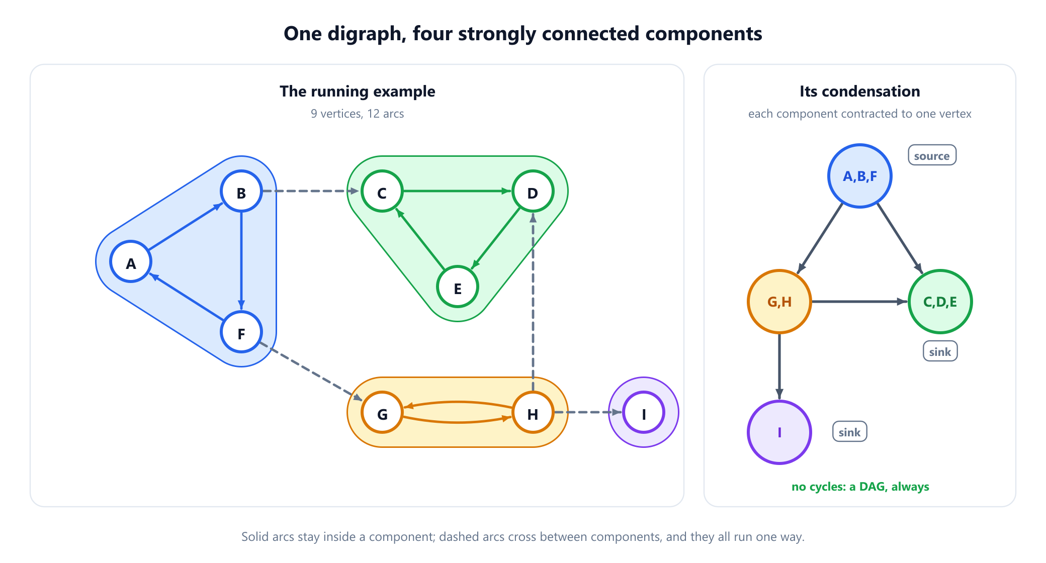
Keep the source and the sinks in mind: the source is where Kosaraju's second pass starts, and a sink is what Tarjan's algorithm reports first.
4. The obvious method, and why it is slow
The definition suggests an algorithm: search from every vertex to get the set R(u) it reaches, and put u and v together exactly when each is in the other's set. On the example the reachable sets hold 49 entries in total: A, B and F reach all nine vertices, G and H reach six, each vertex of {C, D, E} reaches three, and I reaches only itself.
A smarter variant searches forward and backward from one vertex, takes the intersection as its component, removes it and repeats. Both can need a search per vertex, so O(n(n + m)) time, quadratic even on sparse graphs. Early work such as Purdom (1970) and Munro (1971) met SCCs inside transitive closure computations, contracting cycles so that reachability only had to be computed on the smaller condensation. The surprise, established by Tarjan in 1972, is that all components can be found in O(n + m) time, the cost of one search. The trick is not to search more but to read more out of one depth-first search.
5. What depth-first search reveals
A depth-first search stamps each vertex twice: a discovery time when it is first reached and a finish time when all of its outgoing arcs have been explored. Using one counter for both events, a search from A on the example gives:
| Vertex | A | B | C | D | E | F | G | H | I |
|---|---|---|---|---|---|---|---|---|---|
| Discovery | 1 | 2 | 3 | 4 | 5 | 9 | 10 | 11 | 12 |
| Finish | 18 | 17 | 8 | 7 | 6 | 16 | 15 | 14 | 13 |
The search also classifies arcs: a tree arc leads to an undiscovered vertex, a back arc to an unfinished ancestor, a forward arc to a finished descendant, and a cross arc to any other finished vertex. In the example, E → C, F → A and H → G are back arcs, H → D is a cross arc, and the other eight arcs are tree arcs.
Two facts about these numbers carry the whole theory.
Fact 1: each component is a subtree. Let r be the first vertex of a component C to be discovered. Every other vertex of C is then undiscovered and reachable from r inside C, so by the white-path theorem it becomes a descendant of r. Each component is thus a connected piece of the DFS forest below a single root. In the example the roots are A, C, G and I.
Fact 2: finish times respect the condensation. For a component C, let f(C) be the largest finish time of its vertices. If some arc runs from component C to a different component D, then f(C) > f(D). If the search enters C first, all of D is reachable and undiscovered, so it finishes before the root of C does. If it enters D first, nothing in C is reachable from D, or the two would be one component, so all of D finishes before C is even discovered. On the example, f({A,B,F}) = 18, f({G,H}) = 15, f({I}) = 13 and f({C,D,E}) = 8, and every one of the four condensation arcs points from a larger value to a smaller one.
So sorting components by decreasing f gives a topological order of the condensation. It does not follow that the vertex finishing first lies in a sink component. E does in the example, but that is luck. In the three-vertex digraph with arcs a → b, b → a and a → c, a search from a that explores b first finishes b before anything else, yet b lies in the source component {a, b}. The reliable handle is the largest finish time, and Kosaraju's algorithm is built on exactly that.
6. Kosaraju-Sharir: two passes
The algorithm is named after S. Rao Kosaraju, who described it in 1978 without publishing it, and Micha Sharir, who found it independently and published it in 1981; Aho, Hopcroft and Ullman credit both in their 1983 textbook. It is the simplest of the three to explain, because each pass is an ordinary search.
- Pass 1. Run a depth-first search over the whole graph and record the vertices in the order they finish.
- Reverse. Build the reverse graph
GT, with every arc turned around. It has exactly the same components asG, because reversing every path preserves mutual reachability. - Pass 2. Take vertices in decreasing finish time. From each one not yet assigned, search
GTthrough unassigned vertices; everything reached is one component.
Why pass 2 never leaks. The first root lies in the component C with the largest f. A reverse arc from C to another component D is an original arc from D into C, so Fact 2 would give f(D) > f(C), which is impossible. The search therefore reaches all of C and nothing else. Repeat on what remains: each later root has the largest f among unassigned components, so every reverse arc out of its component leads somewhere already assigned.
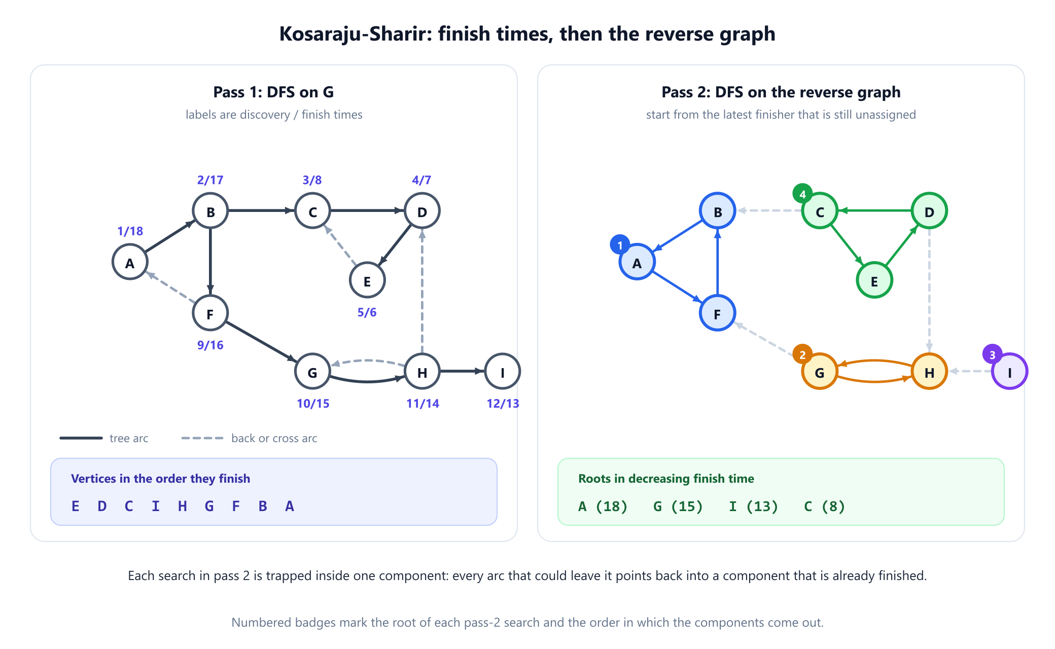
On the example, pass 1 finishes the vertices in the order E, D, C, I, H, G, F, B, A. Pass 2 therefore tries roots in the order A, B, F, G, H, I, C, D, E, skipping any vertex already assigned:
| Root | Finish time | Reverse arcs followed | Reverse arcs into assigned vertices | Component found |
|---|---|---|---|---|
A | 18 | A → F, F → B | none | {A, B, F} |
G | 15 | G → H | G → F | {G, H} |
I | 13 | none | I → H | {I} |
C | 8 | C → E, E → D | C → B, D → H | {C, D, E} |
In the last search, the reverse arcs from C to B and from D to H both lead to assigned vertices, so the search stays inside {C, D, E}, exactly as Fact 2 promises.
The components come out as {A,B,F}, {G,H}, {I}, {C,D,E}, a topological order of the condensation. Kosaraju's algorithm always emits components from sources towards sinks.
A complete implementation follows. Both passes are iterative, so deep graphs do not hit Python's recursion limit. Pass 2 could equally use breadth-first search; only pass 1 needs genuine depth-first finish times.
def kosaraju(graph):
    """Strongly connected components with two depth-first passes."""
    reverse = {u: [] for u in graph}
    for u in graph:
        for v in graph[u]:
            reverse[v].append(u)

    # Pass 1: record vertices in the order they finish.
    order, seen = [], set()
    for root in graph:
        if root in seen:
            continue
        seen.add(root)
        stack = [(root, iter(graph[root]))]
        while stack:
            u, it = stack[-1]
            for v in it:
                if v not in seen:
                    seen.add(v)
                    stack.append((v, iter(graph[v])))
                    break
            else:
                stack.pop()
                order.append(u)

    # Pass 2: search the reverse graph, latest finisher first.
    components, assigned = [], set()
    for root in reversed(order):
        if root in assigned:
            continue
        assigned.add(root)
        component, todo = [], [root]
        while todo:
            u = todo.pop()
            component.append(u)
            for v in reverse[u]:
                if v not in assigned:
                    assigned.add(v)
                    todo.append(v)
        components.append(component)
    return components


graph = {
    'A': ['B'], 'B': ['C', 'F'], 'C': ['D'], 'D': ['E'], 'E': ['C'],
    'F': ['A', 'G'], 'G': ['H'], 'H': ['D', 'G', 'I'], 'I': [],
}
for component in kosaraju(graph):
    print(sorted(component))
# ['A', 'B', 'F']
# ['G', 'H']
# ['I']
# ['C', 'D', 'E']
The cost is two searches plus the reverse graph: O(n + m) time and O(n + m) extra space. That second copy of the arcs is the main practical drawback, unless your graph already stores incoming arcs.
7. Tarjan's algorithm: one pass with low-links
Robert Tarjan's 1972 paper "Depth-first search and linear graph algorithms" found the components in a single search, with no reverse graph, and in the same paper gave linear-time algorithms for biconnected components. Tarjan later shared the 1986 Turing Award with John Hopcroft for their work on the design and analysis of algorithms and data structures, which includes their depth-first search algorithms for biconnectivity and planarity testing.
The algorithm uses Fact 1: each component hangs below a root, so a search that recognises a root as it finishes can report the whole component there and then. Tarjan keeps two numbers per vertex and one stack:
index[u]: the order in whichuwas discovered, 1, 2, 3, and so on.low[u]: the smallest index of a vertex that is still on the stack and can be reached fromu's subtree by following tree arcs and then at most one other arc.- A stack holding every discovered vertex whose component has not been reported yet, in discovery order.
When the search finishes u, it asks one question. If low[u] = index[u], nothing in u's subtree climbs above u, so u is a root, and it pops itself and every vertex above it on the stack as one component. If low[u] < index[u], u belongs to an ancestor's component and stays on the stack.
The update rules, where each arc u → v is examined once:
- If
vis undiscovered, recurse into it, then setlow[u] = min(low[u], low[v]). - If
vis on the stack, setlow[u] = min(low[u], index[v]). The arc leads into a component that is still open. - Otherwise
vbelongs to a component that has already been reported. Ignore the arc.
Here is the full trace on the example. The numbers match the figure below.
| Step | Event | Effect | Stack afterwards (bottom to top) |
|---|---|---|---|
| 1 | Discover A | index = low = 1, push | A |
| 2 | Discover B | index = low = 2, push | A B |
| 3 | Discover C | index = low = 3, push | A B C |
| 4 | Discover D | index = low = 4, push | A B C D |
| 5 | Discover E | index = low = 5, push | A B C D E |
| 6 | Arc E → C, C on the stack | low[E] = min(5, index[C]) = 3 | A B C D E |
| 7 | Back from E to D | low[D] = min(4, low[E]) = 3 | A B C D E |
| 8 | Back from D to C | low[C] = min(3, low[D]) = 3 | A B C D E |
| 9 | C finishes with low = index | Report {C, D, E} | A B |
| 10 | Back from C to B | low[B] = min(2, low[C]) = 2 | A B |
| 11 | Discover F | index = low = 6, push | A B F |
| 12 | Arc F → A, A on the stack | low[F] = min(6, index[A]) = 1 | A B F |
| 13 | Discover G | index = low = 7, push | A B F G |
| 14 | Discover H | index = low = 8, push | A B F G H |
| 15 | Arc H → D, D already assigned | Ignored | A B F G H |
| 16 | Arc H → G, G on the stack | low[H] = min(8, index[G]) = 7 | A B F G H |
| 17 | Discover I | index = low = 9, push | A B F G H I |
| 18 | I finishes with low = index | Report {I} | A B F G H |
| 19 | Back from I to H | low[H] = min(7, low[I]) = 7 | A B F G H |
| 20 | Back from H to G | low[G] = min(7, low[H]) = 7 | A B F G H |
| 21 | G finishes with low = index | Report {G, H} | A B F |
| 22 | Back from G to F | low[F] = min(1, low[G]) = 1 | A B F |
| 23 | Back from F to B | low[B] = min(2, low[F]) = 1 | A B F |
| 24 | Back from B to A | low[A] = min(1, low[B]) = 1 | A B F |
| 25 | A finishes with low = index | Report {A, B, F} | empty |
Two moments matter most. At step 6, the back arc E → C drops low[E] to 3, which travels up to D and stops at C, whose own index is 3, so C reports {C,D,E}. At step 15, the arc H → D is ignored, because D left the stack when its component was reported.
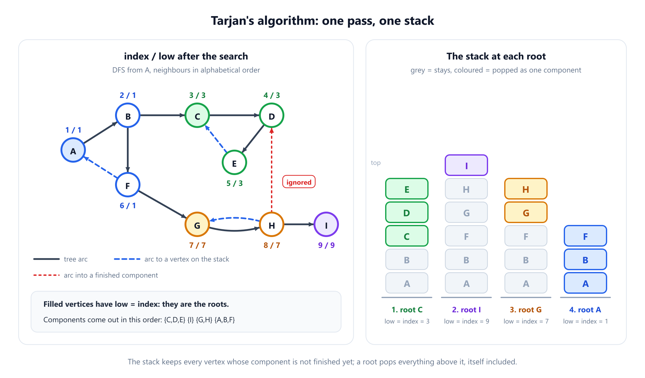
Why the stack holds the right vertices. When a root r finishes, every vertex above it on the stack is an unassigned descendant of r whose low pointed back into the open part of the search, so each can reach r, and r reaches each of them. Conversely, every vertex of r's component is a descendant of r by Fact 1 and cannot have been popped by an earlier root, which would lie in a different component. So the popped set is exactly the component. Tarjan's paper gives the full proof, and Cormen, Leiserson, Rivest and Stein cover both algorithms in their chapter on elementary graph algorithms.
Output order. A component is reported when its root finishes, and by then every component reachable from it has been reported already. So Tarjan's algorithm emits components in reverse topological order, sinks first: {C,D,E}, {I}, {G,H}, {A,B,F}. That is the order dependency resolution wants, and the 2-SAT method in section 12 relies on it.
A direct recursive implementation is short:
def tarjan(graph):
    """Strongly connected components in one depth-first pass."""
    index, low = {}, {}
    stack, on_stack = [], set()
    components = []
    counter = 0

    def strongconnect(u):
        nonlocal counter
        counter += 1
        index[u] = low[u] = counter
        stack.append(u)
        on_stack.add(u)

        for v in graph[u]:
            if v not in index:              # tree edge
                strongconnect(v)
                low[u] = min(low[u], low[v])
            elif v in on_stack:             # edge back into the open part
                low[u] = min(low[u], index[v])
            # otherwise v sits in a finished component: ignore it

        if low[u] == index[u]:              # u is the root of a component
            component = []
            while True:
                w = stack.pop()
                on_stack.discard(w)
                component.append(w)
                if w == u:
                    break
            components.append(component)

    for u in graph:
        if u not in index:
            strongconnect(u)
    return components


graph = {
    'A': ['B'], 'B': ['C', 'F'], 'C': ['D'], 'D': ['E'], 'E': ['C'],
    'F': ['A', 'G'], 'G': ['H'], 'H': ['D', 'G', 'I'], 'I': [],
}
for component in tarjan(graph):
    print(sorted(component))
# ['C', 'D', 'E']
# ['I']
# ['G', 'H']
# ['A', 'B', 'F']
It runs in O(n + m) time, since each vertex is pushed and popped once and each arc examined once, with no reverse graph.
Watch the low-links settle
Draw your own directed graph and step through Tarjan's algorithm arc by arc, or run Kosaraju's two passes on the same graph and compare.
Open the Tarjan SCC Visualizer8. Bugs that survive small tests
Both algorithms are short, and both have well-known mistakes that still produce plausible output on tiny examples. The first three below change the answer on the example graph; the fourth only appears on large inputs.
Dropping the on-stack test
The most common Tarjan bug updates low[u] with index[v] for every discovered v, even one in a component already reported. On the example, the cross arc H → D then pulls low[H] down to index[D] = 4. That value flows up to G, which ends with low[G] = 4, less than its index of 7, so G never recognises itself as a root. G and H stay on the stack and are swept up when A finishes, producing three components instead of four, one of them the false component {A, B, F, G, H}. Yet H cannot reach A.
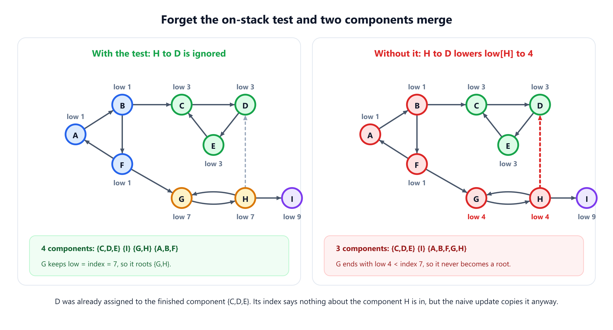
The damage is not always a merge. On the smallest digraph where the bug shows, two vertices and one arc from the second to the first, a search from the first reports it, then visits the second, whose low drops to 1, so the second vertex is never reported at all. Across 20,000 random digraphs with up to eight vertices, the version without the on-stack test returned a wrong partition 9,294 times, so this is not a rare corner case.
Using low[v] instead of index[v] on a non-tree arc
Many implementations write low[u] = min(low[u], low[v]) for every arc into a vertex on the stack, not only for tree arcs. The stored values then stop matching Tarjan's definition: in our test of 20,000 random digraphs they differed from the textbook values on 2,936 graphs. But the root test still gave the correct components on all 20,000, because any vertex on the stack that u can reach and that has a smaller index than u already proves that u is not a root, so which of those indexes gets recorded does not change the test. Write the textbook form anyway, since the proofs and related algorithms such as biconnected components are stated in terms of it, but code using low[v] here is not necessarily producing wrong SCCs.
Kosaraju in the wrong order, or on the wrong graph
Kosaraju's second pass has two silent failure modes. In increasing finish order it starts at E and wanders through D, H, G, F, B, A and C, returning an eight-vertex blob plus {I}. In the right order but on the unreversed graph, the first search from A returns all nine vertices as one component.
Recursion depth
The recursive Tarjan above is correct and still fails in production Python. CPython's default recursion limit is 1,000 frames, and the search recurses once per vertex along a path: the recursive version raised RecursionError on a single cycle of 5,000 vertices. Raising the limit only moves the problem to the operating system's stack. For real inputs, use an explicit stack of iterators:
def tarjan_iterative(graph):
    """Tarjan's algorithm with an explicit call stack (no recursion limit)."""
    index, low = {}, {}
    stack, on_stack = [], set()
    components = []
    counter = 0

    for root in graph:
        if root in index:
            continue
        counter += 1
        index[root] = low[root] = counter
        stack.append(root)
        on_stack.add(root)
        calls = [(root, iter(graph[root]))]

        while calls:
            u, it = calls[-1]
            descended = False
            for v in it:
                if v not in index:
                    counter += 1
                    index[v] = low[v] = counter
                    stack.append(v)
                    on_stack.add(v)
                    calls.append((v, iter(graph[v])))
                    descended = True
                    break
                if v in on_stack:
                    low[u] = min(low[u], index[v])
            if descended:
                continue

            calls.pop()                      # u is finished
            if calls:
                parent = calls[-1][0]
                low[parent] = min(low[parent], low[u])
            if low[u] == index[u]:
                component = []
                while True:
                    w = stack.pop()
                    on_stack.discard(w)
                    component.append(w)
                    if w == u:
                        break
                components.append(component)
    return components


# One cycle of 100,000 vertices: far deeper than Python's recursion limit.
cycle = {i: [i + 1] for i in range(99_999)}
cycle[99_999] = [0]
print(len(tarjan_iterative(cycle)))   # 1
The subtle line follows calls.pop(): a finished vertex folds its low into its parent's, the tree-arc rule the recursive version applies after each call returns.
9. The path-based algorithm
A third linear-time method avoids low-links. Its idea, contracting cycles as the search finds them, is already present in Purdom (1970) and Munro (1971); Dijkstra (1976), Cheriyan and Mehlhorn (1996) and Gabow (2000) refined it into the form usually quoted. It keeps preorder numbers and two stacks:
Sholds every discovered vertex not yet assigned to a component, as in Tarjan's algorithm.Pholds the vertices on the current search path that might still be roots, the boundaries between tentative components.
Each new vertex goes on both stacks. An arc u → v into a discovered but unassigned vertex closes a cycle through the current path, so every boundary on P discovered after v joins one tentative component: P is popped until its top has a preorder number no larger than v's. When u finishes while still on top of P, it is a root: pop it from P, and pop S down to u as one component.
| Event | S (bottom to top) | P (bottom to top) |
|---|---|---|
Discover A (preorder 1) | A | A |
Discover B (preorder 2) | A B | A B |
Discover C (preorder 3) | A B C | A B C |
Discover D (preorder 4) | A B C D | A B C D |
Discover E (preorder 5) | A B C D E | A B C D E |
Arc E → C into an open vertex: pop P above C | unchanged | A B C |
C finishes on top of P: report {C, D, E} | A B | A B |
Discover F (preorder 6) | A B F | A B F |
Arc F → A into an open vertex: pop P above A | unchanged | A |
Discover G (preorder 7) | A B F G | A G |
Discover H (preorder 8) | A B F G H | A G H |
Arc H → G into an open vertex: pop P above G | unchanged | A G |
Discover I (preorder 9) | A B F G H I | A G I |
I finishes on top of P: report {I} | A B F G H | A G |
G finishes on top of P: report {G, H} | A B F | A |
A finishes on top of P: report {A, B, F} | empty | empty |
The merge after F is the whole idea: the arc F → A collapses the boundaries B and F into A, so P shrinks to A alone while S still holds all three vertices. No per-vertex number beyond the preorder index is needed, and components come out in the same reverse topological order as in Tarjan's algorithm. Tarjan and Zwick's 2024 survey in the European Journal of Combinatorics treats both families side by side, together with a bidirectional search method.
10. Which algorithm to use
| Kosaraju-Sharir | Tarjan | Path-based | |
|---|---|---|---|
| Searches | Two | One | One |
| Needs the reverse graph | Yes | No | No |
| Per-vertex data | Visited flag, finish order | Index, low, on-stack flag | Preorder index, component id |
| Stacks | Search stack only | One component stack | Two stacks |
| Output order | Topological (sources first) | Reverse topological (sinks first) | Reverse topological (sinks first) |
| Time | O(n + m) | O(n + m) | O(n + m) |
| Easiest to get wrong | Order of pass 2, forgetting to reverse | On-stack test | Merge condition on P |
All three are linear, so the choice is practical:
- For teaching and interviews, Kosaraju is the easiest to justify on a whiteboard: its correctness argument is Fact 2 alone.
- For production code on large graphs, Tarjan or the path-based algorithm, written iteratively: one search, and no second copy of the arcs.
- For a topological order of the condensation, take Kosaraju's output as it is, or reverse Tarjan's.
- For very large graphs, write the search with an explicit stack in any language, since a recursive search on a path of a million vertices overflows the default stack in C and Java too. When memory is the bottleneck, look at the refinements. Nuutila and Soisalon-Soininen (1994) reduce the stack by not storing vertices that turn out to be single-vertex components, which are common in sparse graphs. Pearce (2016) reduces the worst-case storage of Tarjan's algorithm from about
n(2 + 5w)bits ton(1 + 3w)bits for a word size ofwbits. - For parallel hardware, avoid depth-first search altogether: Reif showed in 1985 that computing the lexicographic DFS order is P-complete, strong evidence that it has no fast parallel algorithm. The forward-backward method of Fleischer, Hendrickson and Pinar (2000) instead picks a pivot, intersects the set it reaches with the set that reaches it to get the pivot's component, and recurses independently on the three remaining parts. Reachability parallelises well, and many parallel SCC implementations build on this idea.
Often you will not write one at all. NetworkX's strongly_connected_components uses a non-recursive version of Tarjan's algorithm with Nuutila's modifications, and SciPy's scipy.sparse.csgraph.connected_components with connection='strong' finds them with a depth-first method whose documentation cites Tarjan and Zwick's survey.
11. Working with the condensation
Finding the components is usually a first step; the next is to build the condensation and solve the real problem on a DAG.
def condensation(graph, components):
    """Contract each component to one vertex. The result is always a DAG."""
    comp = {u: i for i, c in enumerate(components) for u in c}
    dag = {i: set() for i in range(len(components))}
    for u in graph:
        for v in graph[u]:
            if comp[u] != comp[v]:
                dag[comp[u]].add(comp[v])
    return comp, dag


def arcs_to_strongly_connect(dag):
    """Fewest arcs whose addition makes the whole digraph strongly connected."""
    if len(dag) == 1:
        return 0
    has_in = {j for i in dag for j in dag[i]}
    sources = sum(1 for i in dag if i not in has_in)
    sinks = sum(1 for i in dag if not dag[i])
    return max(sources, sinks)


graph = {
    'A': ['B'], 'B': ['C', 'F'], 'C': ['D'], 'D': ['E'], 'E': ['C'],
    'F': ['A', 'G'], 'G': ['H'], 'H': ['D', 'G', 'I'], 'I': [],
}
components = [['C', 'D', 'E'], ['I'], ['G', 'H'], ['A', 'B', 'F']]   # Tarjan's order
comp, dag = condensation(graph, components)
print({i: sorted(dag[i]) for i in dag})
# {0: [], 1: [], 2: [0, 1], 3: [0, 2]}
print(arcs_to_strongly_connect(dag))
# 2
Once you have the condensation, many questions reduce to simple facts about its sources and sinks:
- Is the graph strongly connected? Exactly when there is one component.
- Which vertices reach every vertex? None, unless the condensation has a single source component, in which case exactly its vertices do:
A,BandFin the example. - How many arcs must be added to make the graph strongly connected? If the graph is not already strongly connected, the answer is the larger of the number of source components and the number of sink components, a result of Eswaran and Tarjan (1976). The example has one source and two sinks, so two new arcs suffice and one does not: all 60 possible single arcs leave it disconnected, while 99 of the pairs of arcs work. We also confirmed the formula against exhaustive search on every random digraph with at most five vertices in our test set.
- Dynamic programming over cycles. To find the largest total vertex weight a walk can collect, note that a walk can visit a whole component, so sum the weights per component and run an ordinary longest-path computation on the DAG.
12. Where SCCs are used
2-SAT in linear time
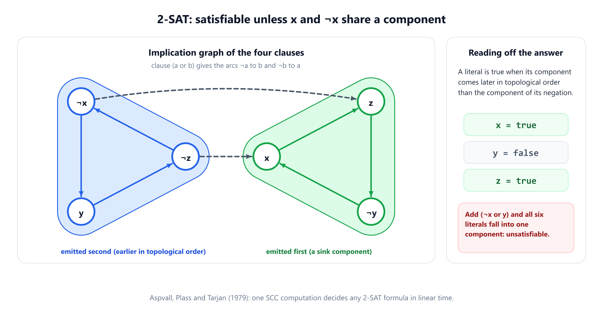
A 2-SAT formula is a conjunction of two-literal clauses, such as (x ∨ y) ∧ (¬x ∨ z). General satisfiability is NP-complete, but Aspvall, Plass and Tarjan showed in 1979 that this case needs only one SCC computation.
Build the implication graph: one vertex per literal, and for each clause (a ∨ b) the two arcs ¬a → b and ¬b → a, since if one literal is false the other must be true. The formula is satisfiable if and only if no variable x shares a component with ¬x, and then setting each literal true when its component comes later in topological order than its negation's satisfies it. With Tarjan's sinks-first output, the literal whose component is reported first wins.
# tarjan(graph) is the function from section 7.


def neg(literal):
    return literal[1:] if literal.startswith('~') else '~' + literal


def solve_2sat(variables, clauses):
    """Aspvall-Plass-Tarjan: 2-SAT via strongly connected components."""
    graph = {lit: [] for x in variables for lit in (x, '~' + x)}
    for a, b in clauses:                 # clause (a or b)
        graph[neg(a)].append(b)          # not a  implies  b
        graph[neg(b)].append(a)          # not b  implies  a

    # Tarjan emits components in reverse topological order.
    rank = {}
    for i, component in enumerate(tarjan(graph)):
        for lit in component:
            rank[lit] = i

    assignment = {}
    for x in variables:
        if rank[x] == rank['~' + x]:
            return None                  # x and not x are equivalent
        assignment[x] = rank[x] < rank['~' + x]
    return assignment


# Three talks, each in the morning (True) or the afternoon (False).
variables = ['x', 'y', 'z']
clauses = [
    ('x', 'y'),     # at least one of x and y is in the morning
    ('x', 'z'),     # at least one of x and z is in the morning
    ('~x', 'z'),    # if x is in the morning, so is z
    ('~y', '~z'),   # y and z are not both in the morning
]
print(solve_2sat(variables, clauses))
# {'x': True, 'y': False, 'z': True}

# Add: if x is in the morning, so is y.
print(solve_2sat(variables, clauses + [('~x', 'y')]))
# None
In the example, three talks are each scheduled in the morning or the afternoon under four constraints. The implication graph splits into two components, {x, z, ¬y} and {¬x, y, ¬z}, and the first is reported first, so x and z are true and y is false, which is the only satisfying assignment. Adding the clause "if x is in the morning, so is y" joins all six literals into a single component, so x and ¬x coincide and the formula has no solution.
The structure of the web
In 2000, Broder and colleagues analysed web crawls of about 200 million pages and 1.5 billion links and found a bow-tie. At its centre was one giant strongly connected component of about 56 million pages, in which every page could reach every other by following links. Around it sat three sets of about 44 million pages each: IN, pages that can reach the core but cannot be reached from it; OUT, pages reachable from the core with no way back; and tendrils, pages hanging off IN or OUT without passing through the core.
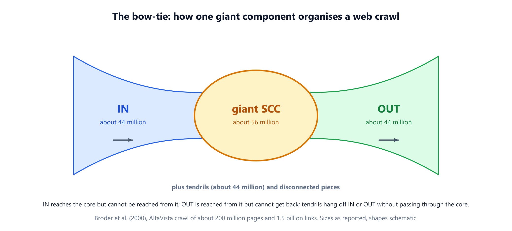
The bow-tie is the condensation seen at a distance: a crawler seeded in OUT never finds the core, and a random surfer in a sink component can never leave by following links, one reason PageRank adds random jumps. The shape has since been reported in other large directed networks, including metabolic networks.
Deadlocks
In a wait-for graph, each process points at the processes holding resources it waits for. Holt's 1972 survey formalised the link with cycles: when every resource has a single unit, the system is deadlocked exactly when the graph has a cycle. A cycle detector says whether a deadlock exists; the SCCs group the processes caught in cycles, since each nontrivial component is a set of processes blocked on one another.
Compilers, builds and packages
Sharir's 1981 paper was titled for its application, data flow analysis. In a call graph, a nontrivial component is a set of mutually recursive functions that an optimiser must analyse together. Build systems and package managers face the same shape: when a dependency graph that should be a DAG is not, the SCCs let the error name every package in each cycle instead of only saying that a cycle exists.
Markov chains
Draw an arc for every transition of a finite Markov chain with positive probability, and the strongly connected components are the chain's communicating classes. The closed classes, which no probability leaves, are exactly the sink components, and in a finite chain their states are the recurrent ones while every other state is transient. The chain is irreducible exactly when the graph is strongly connected.
13. Frequently asked questions
What is a strongly connected component in simple terms?
+
It is a largest possible group of vertices in a directed graph in which you can travel from any vertex to any other and back by following arcs. Every vertex belongs to exactly one such group; a vertex on no cycle forms a group by itself.
What is the difference between Tarjan's and Kosaraju's algorithms?
+
Kosaraju's algorithm runs two depth-first searches, the second on the reversed graph in decreasing finish time, and reports components in topological order. Tarjan's runs one search with an index, a low-link value and a stack, and reports them in reverse topological order. Both take O(n + m) time; Tarjan's needs no reverse graph.
Why does Kosaraju's algorithm need the reversed graph?
+
The vertex with the largest finish time lies in a source component of the condensation, so a forward search from it escapes into every component downstream. In the reversed graph that component has no arcs to unvisited components, so the search stays inside it.
Why does Tarjan's algorithm check whether a vertex is on the stack?
+
A vertex that is discovered but no longer on the stack belongs to a reported component, so an arc into it says nothing about the component being built. Without the check such an arc can lower a low-link value and hide a real root, merging components or leaving vertices unreported.
What is the time complexity of finding strongly connected components?
+
O(n + m) for n vertices and m arcs stored as adjacency lists, for Tarjan's, Kosaraju's and the path-based algorithm alike. With an adjacency matrix the same algorithms take O(n squared) time.
Do strongly connected components exist in undirected graphs?
+
In an undirected graph every edge runs both ways, so the strongly connected components are just the connected components, found by any single search. The undirected problems that need low-link ideas are bridges, articulation points and biconnected components.
How are strongly connected components used to solve 2-SAT?
+
Each clause (a or b) becomes two implications, not a implies b and not b implies a, in a graph with one vertex per literal. The formula is satisfiable exactly when no variable shares a component with its negation, and setting each literal true when its component comes later in topological order than its negation's satisfies it.
14. References
In chronological order.
- Harary, F., Norman, R. Z. and Cartwright, D. (1965). Structural Models: An Introduction to the Theory of Directed Graphs. New York: Wiley.
- Purdom, P. (1970). “A transitive closure algorithm.” BIT Numerical Mathematics, 10(1), 76–94.
- Munro, I. (1971). “Efficient determination of the transitive closure of a directed graph.” Information Processing Letters, 1(2), 56–58.
- Tarjan, R. E. (1972). “Depth-first search and linear graph algorithms.” SIAM Journal on Computing, 1(2), 146–160.
- Holt, R. C. (1972). “Some deadlock properties of computer systems.” ACM Computing Surveys, 4(3), 179–196.
- Dijkstra, E. W. (1976). A Discipline of Programming. Englewood Cliffs: Prentice-Hall.
- Eswaran, K. P. and Tarjan, R. E. (1976). “Augmentation problems.” SIAM Journal on Computing, 5(4), 653–665.
- Aspvall, B., Plass, M. F. and Tarjan, R. E. (1979). “A linear-time algorithm for testing the truth of certain quantified boolean formulas.” Information Processing Letters, 8(3), 121–123.
- Sharir, M. (1981). “A strong-connectivity algorithm and its applications in data flow analysis.” Computers & Mathematics with Applications, 7(1), 67–72.
- Aho, A. V., Hopcroft, J. E. and Ullman, J. D. (1983). Data Structures and Algorithms. Reading: Addison-Wesley.
- Reif, J. H. (1985). “Depth-first search is inherently sequential.” Information Processing Letters, 20(5), 229–234.
- Nuutila, E. and Soisalon-Soininen, E. (1994). “On finding the strongly connected components in a directed graph.” Information Processing Letters, 49(1), 9–14.
- Cheriyan, J. and Mehlhorn, K. (1996). “Algorithms for dense graphs and networks on the random access computer.” Algorithmica, 15(6), 521–549.
- Norris, J. R. (1997). Markov Chains. Cambridge: Cambridge University Press.
- Broder, A., Kumar, R., Maghoul, F., Raghavan, P., Rajagopalan, S., Stata, R., Tomkins, A. and Wiener, J. (2000). “Graph structure in the Web.” Computer Networks, 33(1–6), 309–320.
- Fleischer, L. K., Hendrickson, B. and Pinar, A. (2000). “On identifying strongly connected components in parallel.” In Parallel and Distributed Processing, Lecture Notes in Computer Science 1800, 505–511. Berlin: Springer.
- Gabow, H. N. (2000). “Path-based depth-first search for strong and biconnected components.” Information Processing Letters, 74(3–4), 107–114.
- Sedgewick, R. and Wayne, K. (2011). Algorithms, 4th edition, section 4.2. Upper Saddle River: Addison-Wesley.
- Pearce, D. J. (2016). “A space-efficient algorithm for finding strongly connected components.” Information Processing Letters, 116(1), 47–52.
- Cormen, T. H., Leiserson, C. E., Rivest, R. L. and Stein, C. (2022). Introduction to Algorithms, 4th edition, chapter 20. Cambridge, MA: MIT Press.
- Tarjan, R. E. and Zwick, U. (2024). “Finding strong components using depth-first search.” European Journal of Combinatorics, 119, 103815.