Network Flow and The Max-Flow Min-Cut Theorem

1. What is a Flow Network?

Imagine a complex city water system. You have a main water treatment plant pushing water out, and a main reservoir where all the water eventually ends up. Between them lies a massive network of pipes of varying sizes.

Some pipes are massive water mains (high capacity), while others are small residential pipes (low capacity). The question is: What is the maximum amount of water you can pump from the plant to the reservoir per second without bursting any pipes?

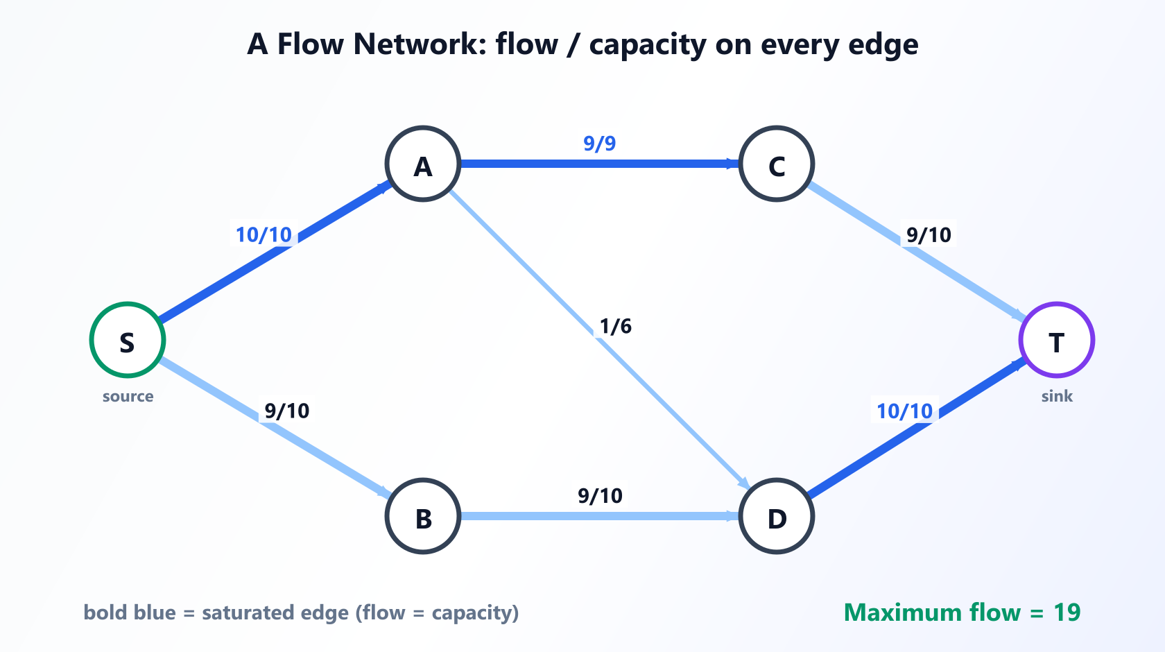
In graph theory, this is modeled as a Flow Network. A flow network is a directed graph where:

• Source (s): The starting node where the "flow" originates (the water plant).
• Sink (t): The destination node where all the "flow" ends up (the reservoir).
• Edges: The connections between nodes (the pipes).
• Capacity (c): The maximum amount of flow an edge can handle (the width of the pipe).

2. The Three Rules of Network Flow

To mathematically define a valid flow through this network, we must follow three absolute rules:

1. Capacity Constraint: The flow on any edge cannot exceed its capacity. If a pipe can hold 10 gallons per second, you can't push 11 gallons through it. Mathematically: 0 ≤ f(u,v) ≤ c(u,v).
2. Conservation of Flow: For every node in the graph (except the Source and the Sink), the total flow entering the node must exactly equal the total flow leaving the node. Nodes don't magically generate or consume water. What goes in must come out.
3. Skew Symmetry (Optional but helpful context): The flow from node U to V is the negative of the flow from V to U. If 5 units flow from U to V, then -5 units flow from V to U.

The goal of the Maximum Flow Problem is to find a valid assignment of flow to every edge that maximizes the total flow leaving the Source s (which, due to conservation of flow, will perfectly equal the total flow arriving at the Sink t).

3. The Ford-Fulkerson Algorithm (Augmenting Paths)

To solve the maximum flow problem, we use the Ford-Fulkerson algorithm, developed in 1956. The logic behind it is delightfully intuitive.

The algorithm works like this:

1. Start with a flow of 0 on all edges.
2. Find a path from the Source to the Sink where every edge in the path has available, unused capacity. This is called an Augmenting Path.
3. Find the edge on this path with the smallest available capacity. This is the "bottleneck" edge.
4. Push an amount of flow equal to the bottleneck capacity along the entire path.
5. Repeat steps 2-4 until no more augmenting paths can be found.

When you can no longer find a path from the Source to the Sink that can accept more flow, you have found the Maximum Flow. But wait, there's a catch!

4. The Secret Weapon: Residual Graphs

If you implement Ford-Fulkerson exactly as described above, you might get the wrong answer. Why? Because you might make a "bad" greedy choice early on, sending flow down a pipe that blocks a much better route later.

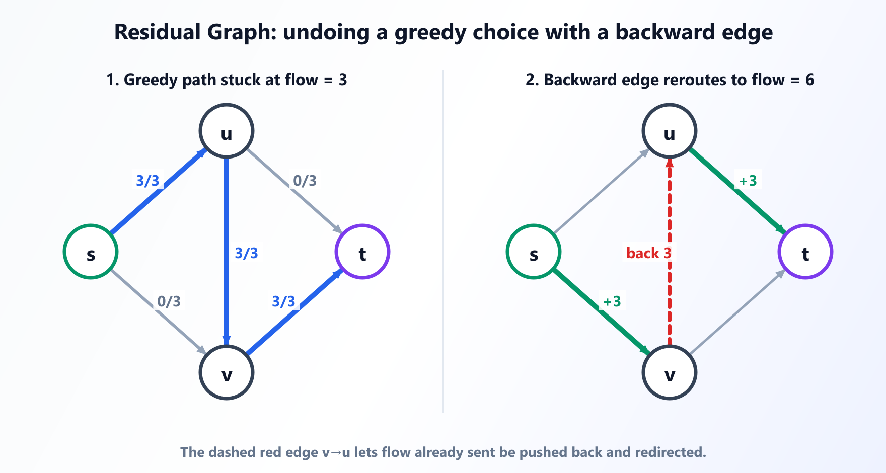
To fix this, Ford-Fulkerson utilizes a brilliant concept called the Residual Graph. The residual graph allows the algorithm to "undo" bad decisions.

Whenever you push X units of flow forward along an edge from U to V, you must add a "backward edge" in the residual graph from V to U with a capacity of X. This backward edge represents your ability to "push back" or cancel out the flow you just sent.

If a future augmenting path utilizes one of these backward edges, it is effectively redirecting the water you previously sent down a different, more optimal pipe. You must always search for your augmenting paths in the Residual Graph, not the original graph.

5. The Max-Flow Min-Cut Theorem

This brings us to one of the most beautiful and profound theorems in all of graph theory: The Max-Flow Min-Cut Theorem.

Imagine you want to completely sabotage the city's water system. You want to sever a set of pipes such that absolutely zero water can reach the reservoir from the treatment plant. Naturally, you want to do this with the least amount of effort, meaning you want to sever pipes whose total combined capacity is as small as possible.

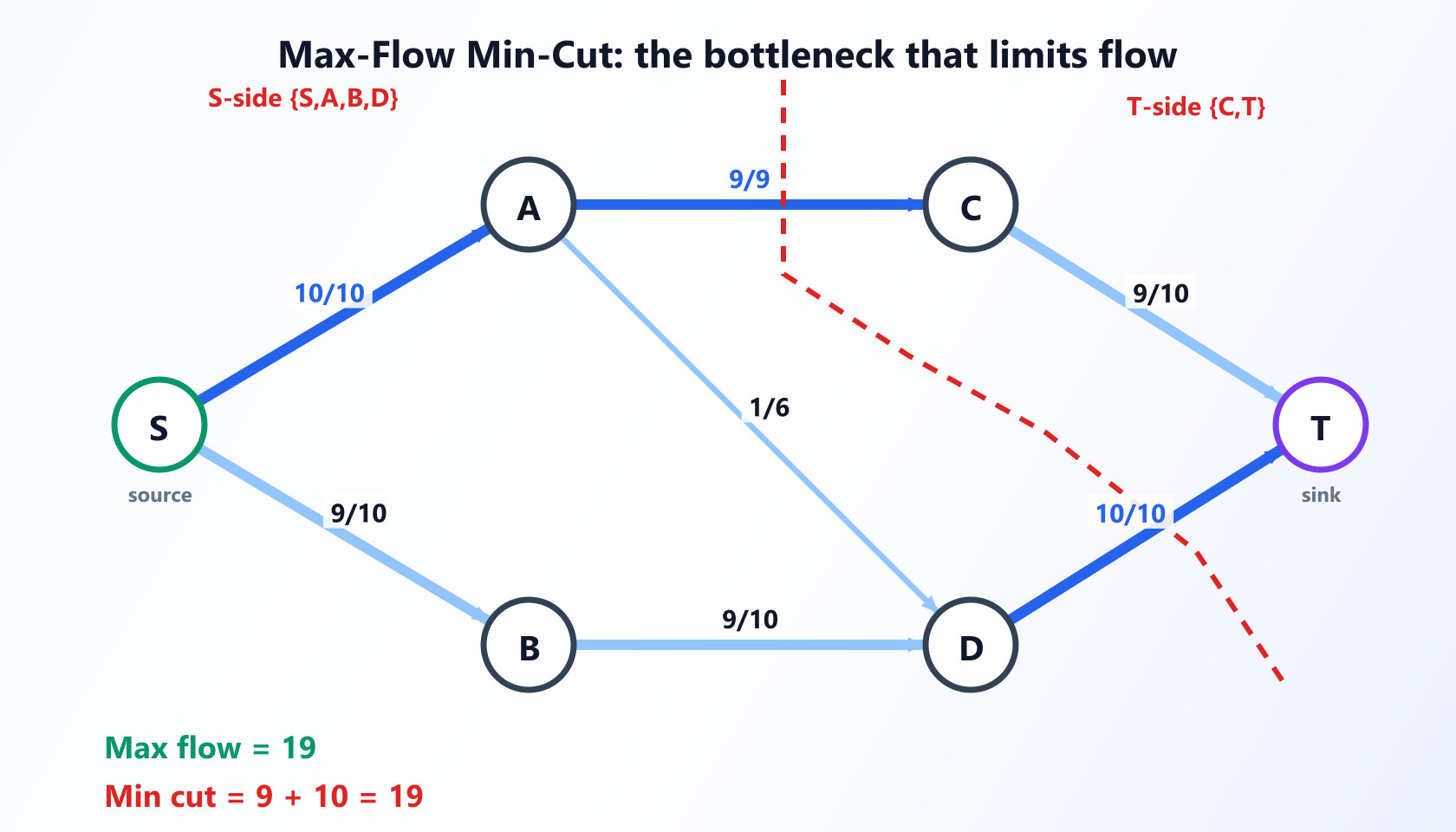
This is called a Cut. An s-t cut partitions the graph's nodes into two sets: one containing the Source (s) and one containing the Sink (t). The capacity of the cut is the sum of the capacities of all edges going from the source set to the sink set.

The Minimum Cut is the cut with the smallest possible total capacity.

The theorem states an incredible equivalence:

The maximum amount of flow you can push through a network is EXACTLY EQUAL to the capacity of the minimum cut.

They are two sides of the exact same coin. The bottleneck that restricts your flow is exactly the same bottleneck you would target to sever the network. By solving for Max-Flow (using Ford-Fulkerson), you are simultaneously finding the exact value of the Min-Cut.

6. Improving Ford-Fulkerson: The Edmonds-Karp Algorithm

Ford-Fulkerson has a flaw: it doesn't tell you how to find the augmenting path. If you just use an arbitrary Depth First Search (DFS), and your graph has very specific edge weights, the algorithm can run incredibly slowly. In fact, with irrational edge capacities, plain Ford-Fulkerson might never even terminate!

In 1972, Jack Edmonds and Richard Karp published a simple but brilliant modification: Always find the shortest augmenting path using Breadth-First Search (BFS).

By forcing the algorithm to find augmenting paths with the fewest number of edges (ignoring capacity), the Edmonds-Karp Algorithm guarantees a polynomial time complexity of O(V * E^2), entirely independent of the actual capacity values on the edges.

7. Real-World Applications

Network flow algorithms aren't just for plumbing. They solve incredibly complex assignment and routing problems in software engineering and operations research.

Maximum Bipartite Matching

Imagine you have 5 job applicants and 5 available jobs. Each applicant is only qualified for certain jobs. How do you assign the maximum number of people to a job they are qualified for?

You can turn this into a Max-Flow problem! Create a "Source" node and connect it to all applicants with capacity 1. Connect the applicants to the jobs they are qualified for with capacity 1. Connect all jobs to a "Sink" node with capacity 1. Run Ford-Fulkerson. The maximum flow will perfectly equal the maximum number of people you can successfully employ.

Image Segmentation in Computer Vision

In computer vision, separating an object (the foreground) from its background is a classic problem. By representing pixels as a graph, where edges represent the color similarity between neighboring pixels, the problem of cutting the foreground from the background can be mapped perfectly to the Minimum-Cut problem.

Sports Elimination

During a baseball season, can you mathematically prove that a team is eliminated from the playoffs, even if they win all their remaining games? By creating a flow network representing the remaining games between all other teams, you can use Max-Flow to prove whether a scenario exists where the team could still win the division.