
Table of Contents
- 1. Introduction to Kruskal's Algorithm
- 2. Why It Works: The Cycle Property
- 3. How the Forest Merges
- 4. Step-by-Step Execution
- 5. Union-Find: The Structure That Makes It Fast
- 6. Implementation and Pseudocode
- 7. Time and Space Complexity
- 8. Kruskal's vs Prim's
- 9. Practical Notes and Common Pitfalls
- 10. Real-World Applications
- 11. Academic Resources and History
- 12. Frequently Asked Questions (FAQ)
1. Introduction to Kruskal's Algorithm
Kruskal's algorithm builds a minimum spanning tree: from a connected, undirected, weighted graph it selects the cheapest set of edges that touches every vertex without forming a cycle. For V vertices that set always contains exactly V - 1 edges.
Where Prim's algorithm grows one connected tree outward from a starting vertex, Kruskal's ignores connectivity almost entirely until the end. It sorts every edge in the graph by weight, walks that list from cheapest to most expensive, and keeps each edge unless doing so would close a cycle. Nothing else is consulted. There is no start vertex and no notion of a frontier.
The consequence is that Kruskal's spends most of its run holding a forest rather than a tree: many small fragments scattered across the graph, growing and merging independently, that only fuse into a single spanning tree with the very last edge it accepts. That difference in shape is what makes it behave differently on sparse graphs, on disconnected input, and under a profiler.
2. Why It Works: The Cycle Property
Prim's correctness rests on a theorem about which edges are safe to accept. Kruskal's spends just as much time rejecting edges, so it is worth stating the companion theorem that justifies throwing one away.
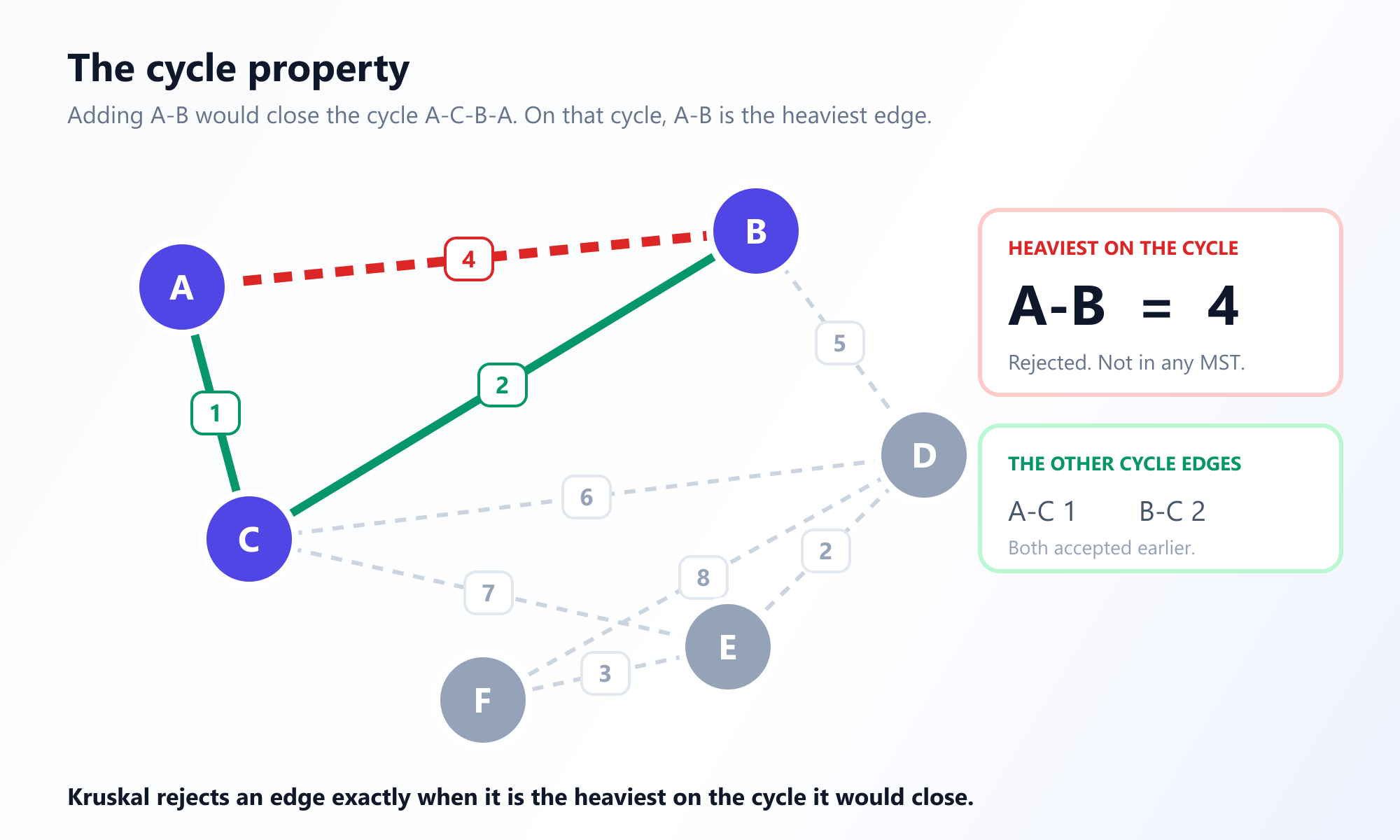
The cycle property. For any cycle in the graph, the maximum-weight edge on that cycle does not belong to the minimum spanning tree, provided it is strictly heavier than every other edge on the cycle. If several edges tie for heaviest, at least one of them can be left out.
The proof mirrors the one for the cut property. Suppose the heaviest edge e on some cycle did belong to a minimum spanning tree T. Removing e from T splits it into two components. The rest of that cycle still runs between those two components, so some other cycle edge f reconnects them. Put f back instead. You have a spanning tree again, and since e was strictly the heaviest, the new tree is strictly lighter, contradicting the assumption that T was minimum.
Now look at what happens when Kruskal's rejects an edge. It reaches edge e and finds that both endpoints already sit in the same fragment. That means a path between them already exists, built entirely from edges the algorithm accepted earlier, which means from edges no heavier than e. Adding e would close a cycle on which e is the heaviest member. By the cycle property, discarding it costs nothing.
The accepted edges are safe for the same reason Prim's are. When an edge joins two different fragments, it is the cheapest remaining edge crossing the cut that separates one fragment from everything else, so the cut property applies unchanged. Kruskal's is greedy in both directions at once, and both directions are theorems.
3. How the Forest Merges
Concretely, the algorithm keeps every vertex in its own fragment to begin with: V fragments, zero edges. Processing the sorted edge list, it asks one question of each edge (u, v):
- Are
uandvalready in the same fragment? If so, the edge would close a cycle. Discard it and move on. - Are they in different fragments? Then accept the edge and merge the two fragments into one.
Each accepted edge reduces the fragment count by exactly one. Starting at V fragments and finishing at one means precisely V - 1 acceptances, which is the stopping condition. Once you have that many, every remaining edge in the list is guaranteed to be rejected, so the loop can exit early.
The whole algorithm therefore reduces to a single data-structure question: how do you test "same fragment?" and "merge these two fragments" quickly, millions of times? That is exactly what union-find provides.
4. Step-by-Step Execution
Take the six-vertex graph used throughout our minimum spanning trees guide. Its nine edges are:
A-B 4    A-C 1    B-C 2
B-D 5    C-D 6    C-E 7
D-E 2    D-F 8    E-F 3
Sorting them by weight gives the order the algorithm will actually walk:
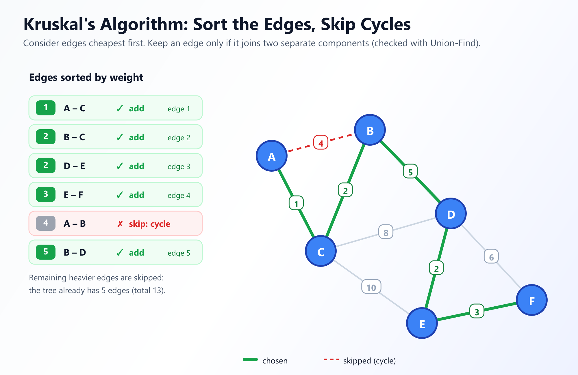
A-C 1 B-C 2 D-E 2 E-F 3 A-B 4 B-D 5 C-D 6 C-E 7 D-F 8Every vertex starts alone, so the forest begins as {A} {B} {C} {D} {E} {F}.
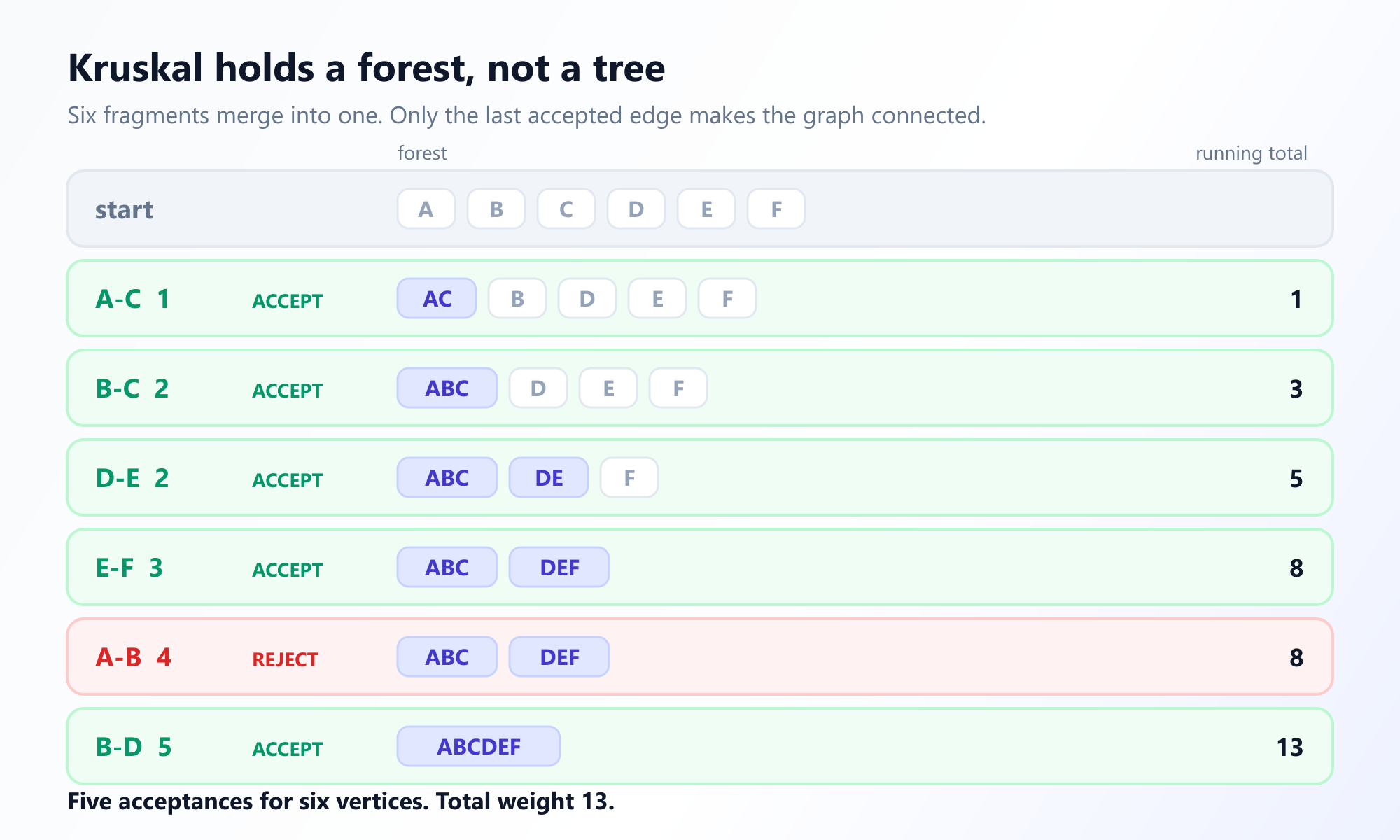
- A-C (1). Accept. Different fragments. Forest becomes
{AC} {B} {D} {E} {F}. Running total 1. - B-C (2). Accept. B is alone, C is with A. Forest becomes
{ABC} {D} {E} {F}. Total 3. - D-E (2). Accept. Note this builds a fragment nowhere near the first one. Forest becomes
{ABC} {DE} {F}. Total 5. - E-F (3). Accept. Forest becomes
{ABC} {DEF}. Total 8. - A-B (4). Reject. A and B are both already in
{ABC}, so this would close the cycle A-C-B-A. Discarded. - B-D (5). Accept. This bridges the two remaining fragments. Forest becomes
{ABCDEF}. Total 13.
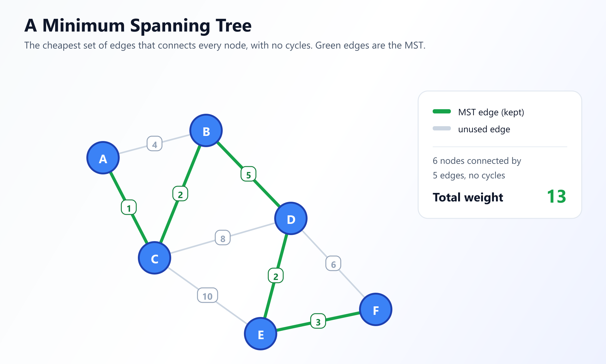
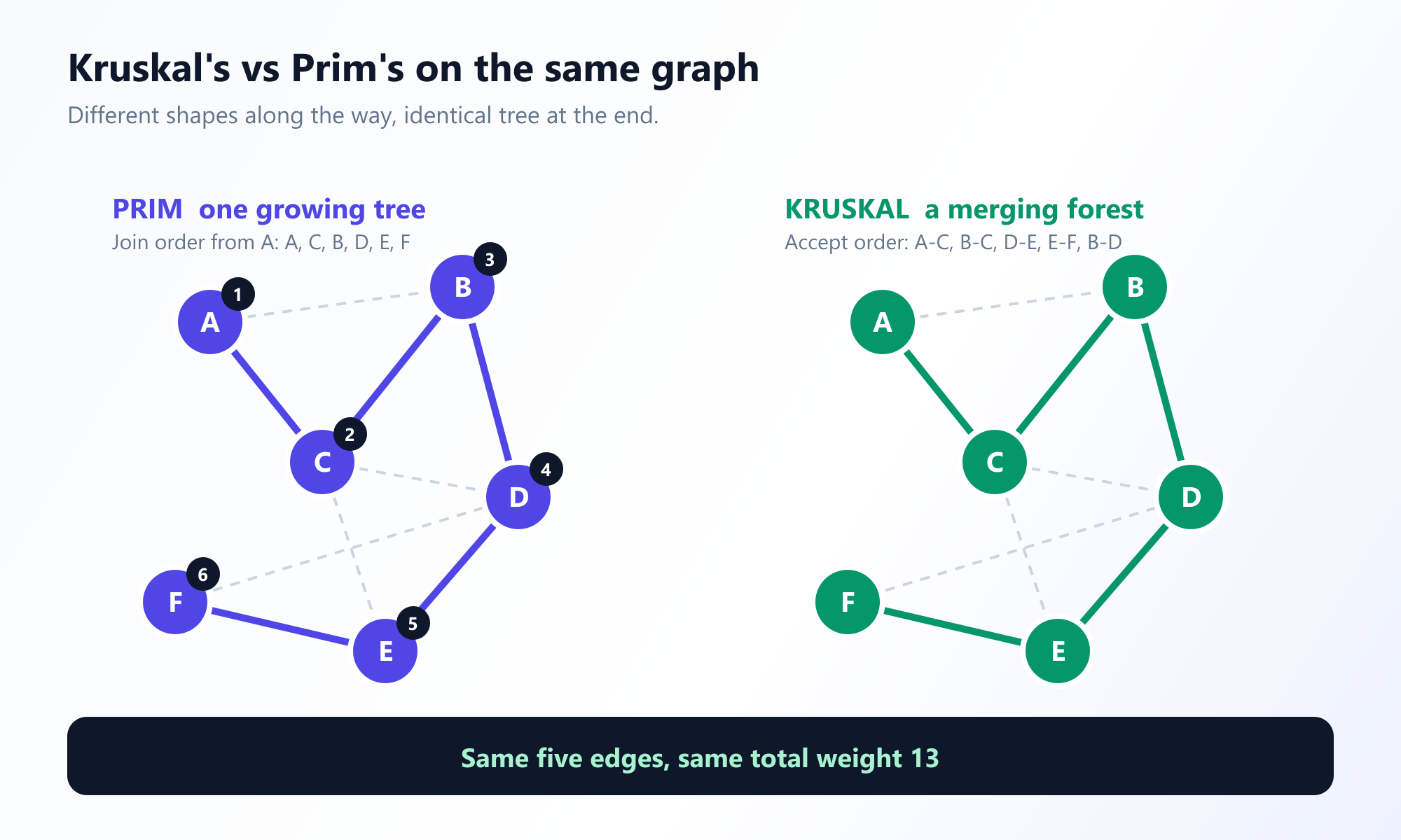
Five edges accepted for six vertices, so the algorithm stops without ever examining C-D (6), C-E (7) or D-F (8). The resulting tree is A-C (1), B-C (2), D-E (2), E-F (3), B-D (5), with total weight 13, exactly the tree Prim's finds on the same graph.
Step 3 is the moment that distinguishes this algorithm. Prim's could not have taken D-E at that point, because neither endpoint touched its growing tree. Kruskal's does not care: it happily starts a second, unrelated fragment on the other side of the graph and worries about connecting them later. And step 5 shows the cycle property in action, rejecting exactly the edge that is heaviest on the cycle it would have created.
5. Union-Find: The Structure That Makes It Fast
The naive way to test whether two vertices are already connected is to run a traversal from one and see whether you reach the other. That costs O(V) per edge and drags the whole algorithm to O(V * E), which is worse than the sort it was supposed to complement.
Union-find, also called the disjoint-set union structure, answers both questions in near-constant time. It maintains each fragment as a tree of parent pointers with one representative element at the root, and exposes two operations:
find(x)returns the representative of x's fragment. Two vertices are in the same fragment exactly when their representatives are identical.union(x, y)merges the two fragments by attaching one root beneath the other.
Two optimisations make it fast enough to disappear from the complexity analysis. Union by rank always attaches the shorter tree under the taller one, keeping the structure from degenerating into a chain. Path compression re-points every node visited during a find straight at the root, so repeated lookups get cheaper as the algorithm runs.
With both applied, a sequence of m operations on n elements costs O(m α(n)), where α is the inverse Ackermann function. It grows so slowly that it is below 5 for any input that fits in the observable universe, so the union-find work in Kruskal's is effectively linear in the number of edges.
6. Implementation and Pseudocode
Because union-find carries the difficulty, the algorithm itself is short.
function Kruskal(V, edges):
    sort edges by weight, ascending
    makeSet(v) for every vertex v      // V singleton fragments
    mst = []

    for each edge (u, v, w) in sorted order:
        if find(u) != find(v):         // different fragments
            union(u, v)
            mst.append((u, v, w))
            if size(mst) == V - 1:     // early exit: tree is complete
                break

    return mst
Two details are worth defending. The break is not required for correctness, since every later edge would be rejected anyway, but on a dense graph it skips most of the list. And dropping the break entirely is not a bug: it is what turns this into a minimum spanning forest algorithm, which is discussed below.
The comparison find(u) != find(v) is the only place cycles are ever considered. There is no explicit cycle detection anywhere, which is the elegance of the approach: connectivity bookkeeping does the job implicitly.
7. Time and Space Complexity
- Sorting:
O(E log E). This dominates everything else. SinceE < V2,log E < 2 log V, so the bound is equivalently writtenO(E log V). - Union-find:
O(E α(V)). At most twofindcalls and oneunionper edge. Effectively linear. - Overall:
O(E log E). The sort and nothing else. - Space:
O(V + E). The parent and rank arrays areO(V); the edge list itself isO(E).
Because the cost is concentrated in one place, the useful optimisations all attack the sort. If the edges arrive pre-sorted, or the weights are small integers that permit a radix or counting sort, the whole algorithm drops to O(E α(V)), which is very close to linear. A partial sort or a lazy heap also helps: you rarely need the full ordering, because the algorithm usually stops long before reaching the heaviest edges.
8. Kruskal's vs Prim's
Both are greedy, both are justified by the same pair of theorems, and on a graph with distinct weights both return the identical tree. The practical differences follow from what each keeps connected.
                 Kruskal                      Prim
structure        forest of fragments          one growing tree
driven by        a sorted edge list           a priority queue
needs            union-find                   a heap (or a V x V scan)
cost             O(E log E)                   O(E log V), or O(V^2) dense
best on          sparse graphs                dense graphs
disconnected     gives a spanning forest      spans one component only
The rule of thumb is density. On a sparse graph, E is small, the sort is cheap, and Kruskal's wins. On a dense graph where E approaches V2, sorting roughly V2 edges costs O(V2 log V), while Prim's with an adjacency matrix runs in a flat O(V2) and takes the lead.
9. Practical Notes and Common Pitfalls
Spanning Forests and Disconnected Graphs
This is where Kruskal's has a genuine structural advantage. Run it on a graph that is not connected and it simply never reaches V - 1 accepted edges. It exhausts the edge list, and what remains is a minimum spanning forest: the minimum spanning tree of each connected component, computed in one pass with no special handling.
Prim's cannot do this from a single start. Launched at one vertex, it spans that vertex's component and stops, silently returning a tree that looks valid but covers only part of the graph. Recovering the rest means detecting the shortfall and restarting from an unvisited vertex, once per component.
The count is also the diagnostic. If Kruskal's finishes having accepted V - 1 edges the graph was connected; if it accepted V - k, the graph had k components. Connectivity information falls out of the algorithm for free.
Maximum Spanning Tree
Sort descending instead of ascending and every line of the algorithm still applies. The cycle property flips to a cut property argument on negated weights, and you get the heaviest spanning tree. Negating the weights and running the algorithm unchanged works equally well.
Reverse-Delete
The mirror image of Kruskal's: sort edges from heaviest to lightest and delete each one unless deleting it would disconnect the graph. It is justified by the same cycle property read backwards, and it produces the same tree. It is rarely used because the connectivity test after each deletion is far more expensive than a union-find query.
Tied Weights
When several edges share a weight the graph can have more than one minimum spanning tree, and which one you get depends on how your sort orders the ties. The example above contains such a tie: B-C and D-E both weigh 2. All the resulting trees are equally optimal, so any test that compares against a fixed edge list is fragile. Compare total weight instead.
Self-Loops and Parallel Edges
A self-loop always fails the find(u) != find(v) test and is discarded automatically, so it needs no special handling. Among parallel edges, the cheapest is reached first and accepted, and the rest are then rejected as cycles. Kruskal's is unusually forgiving about messy input.
10. Real-World Applications
Network and Infrastructure Design
The original motivation: connect a fixed set of sites with the least total cable, pipe or track. Kruskal's edge-centric view fits naturally when the input is already a list of candidate links with costs, which is how such data usually arrives. A tree is only the starting point for a real network, though: every link in it is a single point of failure, and our guide to network design for telecom and utilities shows how to price the extra links that make it survive a cable cut.
Hierarchical Clustering
Run Kruskal's and record the order in which fragments merge, and you have performed single-linkage agglomerative clustering. The sequence of merges is precisely the dendrogram, and stopping early at V - k edges leaves exactly k clusters. This equivalence is why minimum spanning trees show up so often in unsupervised learning.
Image Segmentation
Treating pixels as vertices and intensity differences as edge weights, the Felzenszwalb-Huttenlocher segmentation algorithm is essentially Kruskal's with a merge predicate that compares internal fragment variation against the edge weight.
Circuit and Layout Design
Minimising total wire length between fixed pads is an MST problem, and the edge list of candidate routes is naturally what a router already has to hand.
11. Academic Resources and History
Unlike Prim's algorithm, which was discovered independently at least three times, this one has a clean attribution.
- Joseph B. Kruskal (1956) published it in a three-page note, On the shortest spanning subtree of a graph and the traveling salesman problem, in the Proceedings of the American Mathematical Society. The paper appeared a year before Prim's and thirty years after Borůvka's.
- Otakar Borůvka (1926) had posed and solved the minimum spanning tree problem decades earlier, while planning rural electrification in Moravia.
- Robert Tarjan (1975) proved the near-constant amortised bound for union-find with union by rank and path compression, which is what pins the non-sorting part of Kruskal's cost to
O(E α(V)).
For the full attribution history of the problem, see Graham and Hell. For rigorous proofs of the cut and cycle properties and of both algorithms, the standard reference is Cormen, Leiserson, Rivest and Stein, Introduction to Algorithms, in the chapter on minimum spanning trees. Full citations appear at the end of this article.
Frequently Asked Questions
Why is it safe for Kruskal's algorithm to reject an edge?
Because of the cycle property: the heaviest edge on any cycle can be left out of the minimum spanning tree. When Kruskal's rejects an edge, both endpoints are already in the same fragment, which means a path between them already exists built from edges it accepted earlier, and therefore from edges no heavier than this one. The rejected edge is the heaviest on the cycle it would have closed, so discarding it costs nothing.
Why does Kruskal's algorithm need union-find?
The algorithm must ask, for every edge, whether its two endpoints are already connected. Answering that with a graph traversal costs O(V) per edge and would dominate the whole running time. Union-find answers it in near-constant time using union by rank and path compression, giving O(E alpha(V)) for all the connectivity work, where alpha is the inverse Ackermann function and is below 5 for any practical input.
When should I use Kruskal's algorithm instead of Prim's?
Prefer Kruskal's on sparse graphs, when the input already arrives as an edge list, or when the graph may be disconnected. Its cost is dominated by sorting at O(E log E), which is cheap when E is small, and on a disconnected graph it naturally produces a minimum spanning forest in one pass. Prefer Prim's on dense graphs, where an adjacency-matrix implementation runs in a flat O(V^2) and avoids sorting roughly V squared edges.
Watch Kruskal accept and reject edges
Sort the edges, then watch union-find wave each one through or turn it away. Run Kruskal on a live graph, step by step.
Open the Kruskal Visualizer