Bellman-Ford Algorithm Explained

Mohammed Islam Hadjoudj

Expert Operations Research Engineer

1. Introduction to the Bellman-Ford Algorithm

The Bellman-Ford algorithm is one of the most foundational algorithms in graph theory. Named after its pioneers, Richard Bellman and Lester Ford Jr., who published it in the late 1950s, this algorithm solves the single-source shortest path problem. That means it finds the shortest path from one starting node to all other nodes in a weighted graph.

If you're familiar with Dijkstra's algorithm, you might wonder: "Why do we need another algorithm for the exact same problem?" The answer lies in versatility. While Dijkstra's algorithm is faster and highly efficient for graphs where all edge weights are positive (like physical road networks), it completely breaks down when introduced to negative edge weights. Bellman-Ford, on the other hand, embraces negative weights and provides a robust mechanism to handle them, ensuring accurate shortest path calculations even in complex economic or network scenarios.

Furthermore, Bellman-Ford has a unique superpower: it can detect negative cycles. A negative cycle is a loop in a graph where the sum of the edge weights is less than zero. If such a cycle exists, the concept of a "shortest path" becomes meaningless because one could theoretically traverse the cycle infinitely to achieve a path length of negative infinity. Bellman-Ford detects this anomaly and alerts you to it, making it an indispensable tool for anomaly detection in various fields, including financial arbitrage.

2. The Problem with Dijkstra's: Negative Weights

To truly appreciate the necessity of the Bellman-Ford algorithm, we must first examine the critical limitation of Dijkstra's algorithm.

Dijkstra's algorithm operates on a greedy principle. It maintains a set of unvisited nodes and, at each step, selects the node with the smallest known distance from the source. Once a node is selected, Dijkstra's algorithm considers its shortest distance "finalized" and never revisits it to update its distance. This assumption works perfectly when all edge weights are positive because adding another edge to a path will always increase the total path length. Therefore, no later discovered path could possibly be shorter than the one currently finalized.

However, what happens when we introduce a negative edge weight?

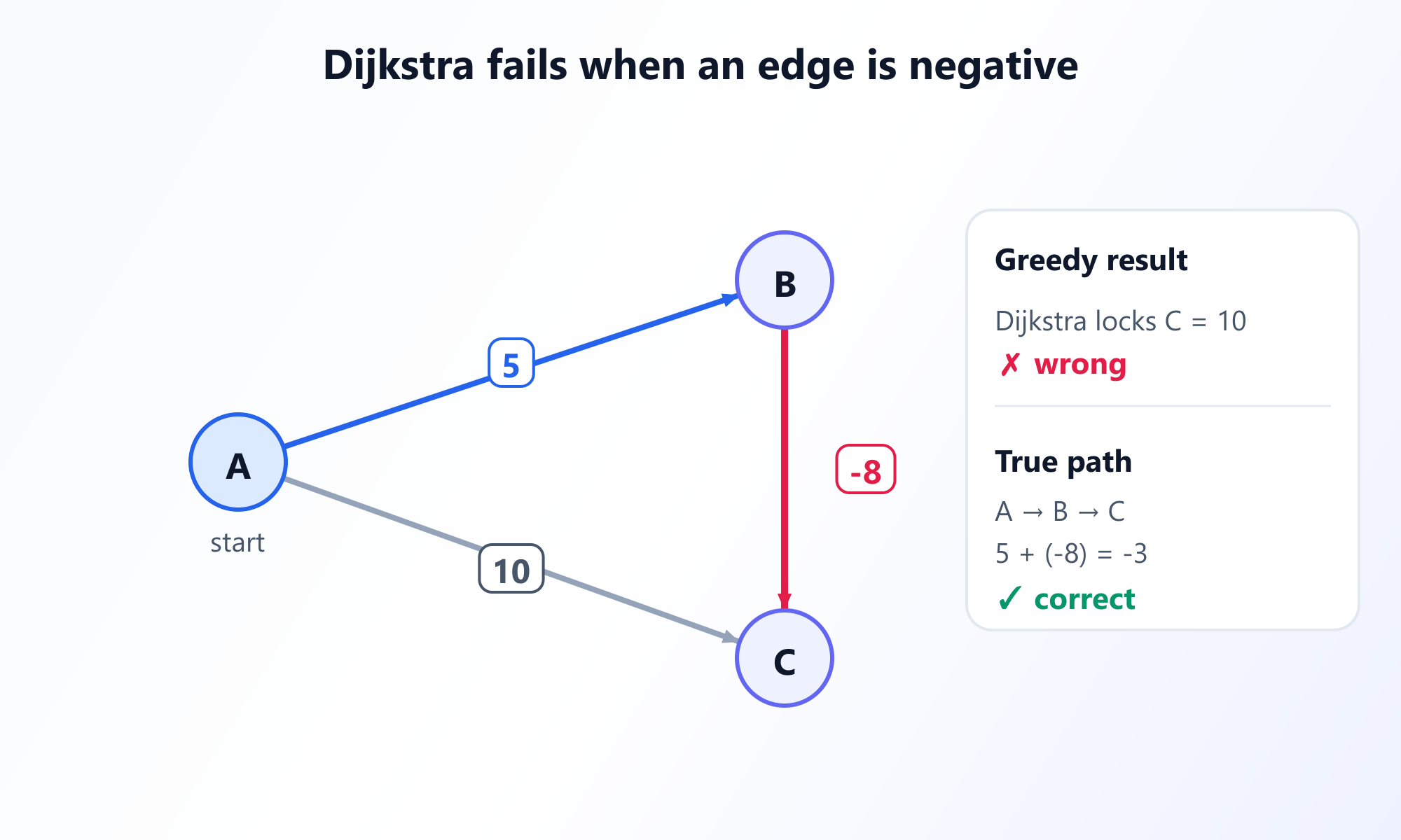
Consider a simple graph with three nodes: A, B, and C. The starting node is A.

• The edge from A to B has a weight of 5.
• The edge from A to C has a weight of 10.
• The edge from B to C has a weight of -8.

If we run Dijkstra's algorithm from A, it will first explore the neighbors B (distance 5) and C (distance 10). The next node to be finalized is B, because 5 is smaller than 10. The shortest distance to B is now locked in as 5. Next, it looks at edges from B. It sees the edge from B to C with weight -8. The new path to C is A -> B -> C, which has a total weight of 5 + (-8) = -3. But Dijkstra's algorithm is greedy; if it had finalized C before realizing there was a negative edge, or if the graph was more complex, Dijkstra's would fail to update C properly and return an incorrect result. In more complex graphs, Dijkstra's greedy assumption that "longer paths can't become shorter" falls apart.

This is where Bellman-Ford shines. It abandons the greedy approach and instead systematically relaxes all edges multiple times, guaranteeing that even if a negative edge provides a shorter shortcut later in the process, the algorithm will correctly identify and update the shortest path.

3. The Danger of Negative Cycles

A negative cycle is a closed loop in a graph where the sum of the weights of the edges making up the cycle is less than zero. This concept is fundamental to why Bellman-Ford is designed the way it is.

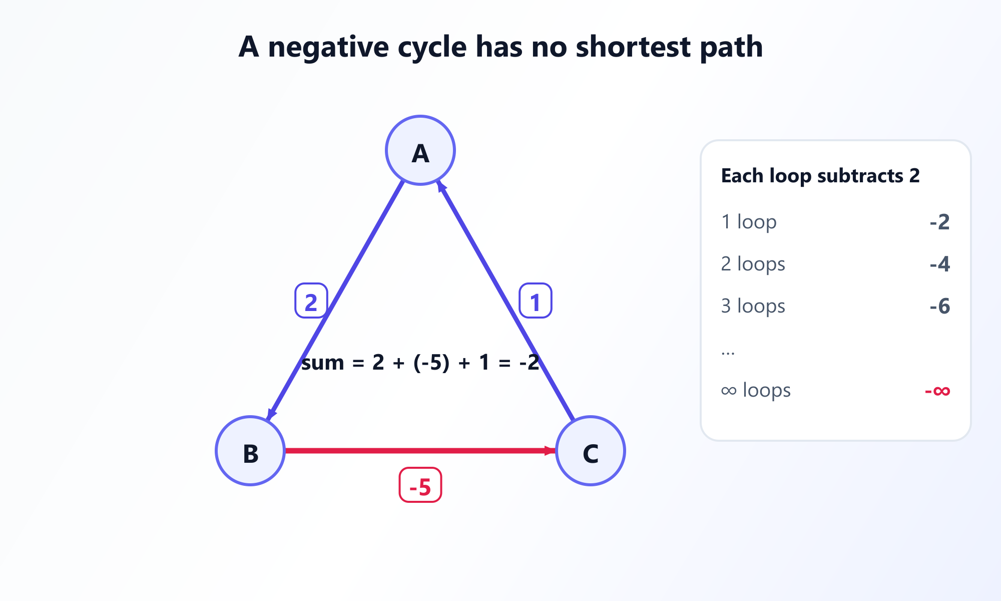
Imagine a graph with nodes A, B, and C forming a triangle. The edge weights are A to B (2), B to C (-5), and C to A (1). The total weight of this cycle is 2 + (-5) + 1 = -2. If you want to find the shortest path from A to anywhere else, you could simply travel around this cycle infinitely. Each time you complete the loop, your total path distance decreases by 2. After one loop, the distance is -2. After ten loops, the distance is -20. As you approach infinity, the shortest path becomes negative infinity.

In the presence of a negative cycle that is reachable from the source node, the shortest path problem has no solution. Standard algorithms would get trapped in an infinite loop, constantly trying to find a "shorter" path. Bellman-Ford elegantly avoids this infinite loop and explicitly detects the cycle's presence.

4. Core Concept: Edge Relaxation

The foundation of the Bellman-Ford algorithm is a process called Edge Relaxation. This is the mechanism by which the algorithm updates the shortest known distance to a node.

Let's define two arrays (or dictionaries):

• distance[]: This stores the shortest known distance from the starting node to every other node. Initially, the distance to the start node is 0, and the distance to all other nodes is set to infinity (∞).
• predecessor[] (optional but useful): This stores the node that comes immediately before a given node on the shortest path. This is used to reconstruct the actual path once the algorithm finishes.

The relaxation operation for an edge from node u to node v with weight w is defined as follows:

if distance[u] + w < distance[v]:
    distance[v] = distance[u] + w
    predecessor[v] = u

In plain English: "If the known distance to node u plus the weight of the edge from u to v is smaller than the currently known shortest distance to node v, then we have found a better path! Update the shortest distance to v."

The Bellman-Ford algorithm simply iterates through all the edges in the graph and attempts to relax them over and over again.

5. Step-by-Step Execution of Bellman-Ford

Now, let's walk through the exact steps of the algorithm.

Let V be the number of vertices (nodes) in the graph, and E be the number of edges. The algorithm proceeds in three main phases.

Phase 1: Initialization

Initialize the distance array. Set the distance to the starting node to 0, and the distance to all other nodes to infinity. This represents that initially, we don't know how to reach any node other than the start.

Phase 2: Repeated Relaxation

This is the core of the algorithm. We must relax all edges in the graph, and we must do this V - 1 times.

Why exactly V - 1 times? Consider a graph with V nodes. The longest possible simple shortest path (a path without any cycles) between any two nodes can have at most V - 1 edges. In the worst-case scenario, it takes one full iteration over all edges to guarantee that paths of length 1 edge are correct. It takes two iterations to guarantee paths of length 2 edges are correct, and so on. Therefore, after V - 1 iterations, if there are no negative cycles, we are guaranteed to have found the absolute shortest path to every node, regardless of the order in which we process the edges.

1. Start a loop that runs V - 1 times.
2. Inside this loop, iterate through every single edge in the graph.
3. For each edge (u, v) with weight w, attempt to relax it: If distance[u] + w < distance[v], update distance[v].

Phase 3: Negative Cycle Detection

After completing Phase 2, we have the shortest distances, assuming no negative cycles exist. To check for negative cycles, we run one final, additional iteration over all the edges.

1. Iterate through every edge (u, v) with weight w one last time.
2. Attempt to relax it. If distance[u] + w < distance[v] is STILL true, it means we found a path that is even shorter after V - 1 edges.
3. This is mathematically impossible for a simple path. The only explanation is that we have entered a negative weight cycle that allows us to infinitely reduce the distance. If this occurs, the algorithm terminates and reports that a negative cycle exists.

6. Implementation and Pseudocode

The beauty of Bellman-Ford lies in its simplicity. The implementation is remarkably straightforward, often just a few nested loops. Here is the standard pseudocode:

function BellmanFord(Graph, source):
    // Phase 1: Initialization
    distance = array of size |V|, filled with Infinity
    predecessor = array of size |V|, filled with Null
    distance[source] = 0

    // Phase 2: Relax all edges |V| - 1 times
    for i from 1 to |V| - 1:
        for each edge (u, v) with weight w in Graph:
            if distance[u] + w < distance[v]:
                distance[v] = distance[u] + w
                predecessor[v] = u

    // Phase 3: Check for negative-weight cycles
    for each edge (u, v) with weight w in Graph:
        if distance[u] + w < distance[v]:
            return "Error: Graph contains a negative-weight cycle"

    return distance, predecessor

This code is language-agnostic and translates easily into Python, C++, Java, or JavaScript.

7. Time and Space Complexity Analysis

While Bellman-Ford is highly versatile, it comes with a performance cost compared to greedy algorithms.

• Time Complexity: The algorithm runs a loop V - 1 times, and inside that loop, it iterates over all E edges. Therefore, the time complexity for Phase 2 is O(V * E). The cycle detection phase takes O(E). The overall time complexity is O(V * E). In a dense graph where E is close to V², the complexity approaches O(V³). This makes it significantly slower than Dijkstra's algorithm, which can achieve O(V log V + E) with a Fibonacci heap.
• Space Complexity: The algorithm only needs to store the distance array and the predecessor array, both of size V. It also needs to store the graph itself. Therefore, the auxiliary space complexity is O(V).

Because of its O(V * E) time complexity, Bellman-Ford is typically used only when necessary—that is, when negative weights are present or negative cycle detection is a strict requirement. For strictly positive graphs, Dijkstra's is the preferred choice.

8. Real-World Applications

Despite being slower than Dijkstra's, Bellman-Ford has profound real-world applications, particularly in networking and finance.

Routing Information Protocol (RIP)

In computer networking, routing protocols determine how data packets travel across the internet. One of the earliest and most famous protocols, the Routing Information Protocol (RIP), is a distance-vector routing protocol that relies heavily on a distributed variant of the Bellman-Ford algorithm.

In this distributed setup, routers do not have a complete map of the entire network. Instead, each router only knows about its immediate neighbors. Routers periodically share their routing tables (their known shortest distances to various destinations) with their neighbors. When a router receives an update, it uses the Bellman-Ford relaxation equation to update its own routing table. Over time, this information propagates through the network, allowing all routers to converge on the shortest paths.

Financial Arbitrage Detection

Arbitrage is the practice of taking advantage of a price difference between two or more markets. In the foreign exchange (Forex) market, currency exchange rates fluctuate. An arbitrage opportunity exists if you can start with a currency, trade it through a sequence of other currencies, and end up with more of your original currency than you started with, without taking any market risk.

We can model currency exchange rates as a graph where nodes are currencies (USD, EUR, GBP, etc.) and edges represent the exchange rate. Because we multiply exchange rates rather than add them, we can take the negative logarithm of the exchange rates to convert the problem into an additive one. An arbitrage opportunity (where the product of rates > 1) transforms into a negative cycle in our modified graph. Running Bellman-Ford on this graph will detect these negative cycles, instantly identifying profitable arbitrage loops for algorithmic traders.

9. Academic Resources and History

The Bellman-Ford algorithm is sometimes referred to as the Bellman-Ford-Moore algorithm to recognize the independent contributions of these three computer scientists:

• Alfonso Shimbel (1955): Originally proposed the algorithm, though it was less widely popularized.
• Edward F. Moore (1959): Published a variation of the algorithm in "The shortest path through a maze" (Proceedings of the International Symposium on the Theory of Switching).
• Richard Bellman (1958): Formalized it in "On a routing problem" (Quarterly of Applied Mathematics).
• Lester Ford Jr. (1956): Developed the foundational concepts in "Network Flow Theory" (RAND Corporation Paper).

This algorithm laid the groundwork for dynamic programming, a method famously pioneered by Richard Bellman himself, leading to widespread applications across mathematics, economics, and computer science.