
Table of Contents
- 1. Why the sequence is where the week's money goes
- 2. What a production schedule costs
- 3. The week used throughout
- 4. Step one: the schedule as a graph
- 5. How schedules get made without optimisation
- 6. Colour changes: a travelling salesperson inside the paint line
- 7. Smarter heuristics: NEH and local search
- 8. The exact answer
- 9. A rush order arrives
- 10. Is a Saturday shift worth it?
- 11. Finishing first is not finishing cheapest
- 12. Job shops and the disjunctive graph
- 13. What is easy, what is hard
- 14. What the model leaves out
- 15. From spreadsheet to optimisation
- 16. Mistakes that quietly cost money
- 17. Frequently asked questions
- 18. References
1. Why the sequence is where the week's money goes
In most small and mid-sized factories the production schedule lives in a spreadsheet. Orders are typed in as they arrive, a planner reorders a few rows when a customer calls, and the shop floor works down the list. It is flexible, familiar and free, and it hides a question that decides a surprising share of the week's costs: in what order should the orders run?
The order matters because work waits. An order that runs early finishes early, and every order behind it finishes a little later. On a line with several machines the effects compound, colour or tooling changes add time that depends on which job follows which, and the difference between two sequences of the same orders can be the difference between delivering on time within the normal week and paying for overtime and late deliveries.
Scheduling theory is one of the founding subjects of operations research. Selmer Johnson solved the two-machine case in 1954, James Jackson and Wayne Smith gave the classic rules for a single machine in 1955 and 1956, and in 1964 Bernard Roy and Bertrand Sussmann described job shop scheduling with a graph that is still the basis of modern solvers. Michael Pinedo's textbook covers the field as it stands today.
This article takes one realistic week on a three-machine line, eight customer orders with due dates, late penalties and paint colours, and sequences it seven ways, from the spreadsheet's order to a proven optimum found by checking every possible sequence. Every number below was computed by solving the model, not estimated.
2. What a production schedule costs
For a fixed set of orders the materials and the processing hours are the same whatever the sequence. What the sequence changes is two lines on the bill:
- Late penalties. Each order has a due time and a cost for every hour it is late, which stands for contractual penalties, expediting, lost goodwill or a missed truck. Orders for important customers carry a higher rate.
- Overtime. The line runs two 8-hour shifts, 40 hours in the week used here. Every hour the line keeps running after that costs $450 in overtime for the crew.
These figures are illustrative rather than taken from any particular plant, but the structure is typical, and it explains why sequencing is hard to do by eye: moving one order earlier can save its penalty and cost another order's, and a sequence that finishes within the week can still make the wrong orders late.
3. The week used throughout
Every order passes through the same three machines in the same order: Cut, then Weld, then Paint. Orders cannot overtake each other between machines, so a schedule is simply a sequence of the eight orders. This is a permutation flow shop.
| Order | Cut, h | Weld, h | Paint, h | Due at hour | Penalty per late hour | Colour |
|---|---|---|---|---|---|---|
| A | 3 | 7 | 4 | 28 | $120 | Grey |
| B | 7 | 6 | 2 | 34 | $80 | Grey |
| C | 3 | 5 | 3 | 25 | $120 | White |
| D | 3 | 3 | 2 | 42 | $80 | Grey |
| E | 2 | 3 | 4 | 45 | $150 | White |
| F | 6 | 3 | 5 | 45 | $40 | Red |
| G | 7 | 4 | 5 | 24 | $100 | Grey |
| H | 5 | 5 | 3 | 28 | $120 | Black |
The orders need 100 machine-hours in total, and the paint line also has to be cleaned whenever the colour changes. Cleaning takes longer going from a dark colour to a light one:
| Cleaning hours, from (row) to (column) | White | Grey | Red | Black |
|---|---|---|---|---|
| White | 0 | 0.5 | 1 | 1 |
| Grey | 2 | 0 | 1 | 1 |
| Red | 3 | 2.5 | 0 | 1 |
| Black | 4 | 3.5 | 3 | 0 |
The paint line starts the week clean, as if it had just painted white. Eight orders can be arranged in 8! = 40,320 different sequences, and the task is to find the cheapest.
4. Step one: the schedule as a graph
Once a sequence is fixed, every start and finish time follows from two rules: an operation cannot start until the same order has left the previous machine, and it cannot start until the order ahead of it on the same machine has finished. Both are arcs in a graph. Draw one node for each order on each machine, an arc along each row for "the order ahead on this machine" and an arc down each column for "the previous step of this order", and weight each node by its processing time.
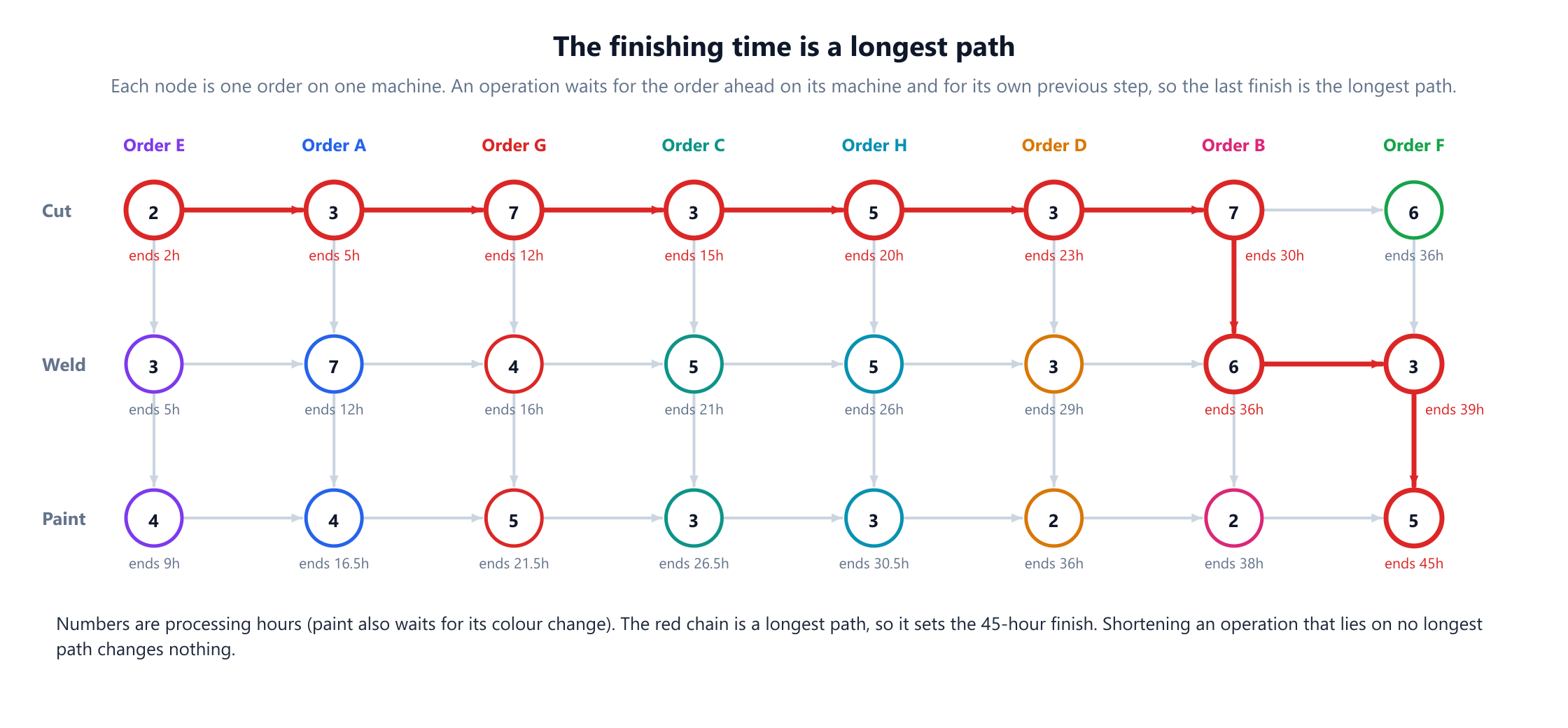
The graph is a directed acyclic graph, and the time the last order leaves the paint line, the makespan, is the length of the longest path through it, with each colour change added in front of its paint operation. For the optimal sequence that is 45 hours. The operations on a longest path form a critical path, exactly as in the critical path method for projects: shortening an operation that lies on no longest path cannot bring the finish forward, and making a critical operation longer delays everything.
On this schedule there is a tie. Order F's cut and order B's weld both finish at 36 hours, so two longest paths reach F's weld at the same moment, and speeding up only one of them would not help. Ties like this are why spotting the bottleneck by eye is unreliable, and why computing the longest paths is worth the few milliseconds it takes. Longest paths in an acyclic graph are found in one pass in topological order.
5. How schedules get made without optimisation
Four common ways to sequence the week make a fair baseline, because each is what a sensible planner might do.
The spreadsheet order. Run the orders in the order they were entered, A to H. It finishes at 52 hours, 12 hours into overtime, and orders G and H are each 24 hours late. Cost: $10,800, split evenly between $5,400 of penalties and $5,400 of overtime. Of all 40,320 possible sequences, the median costs $10,110, so the order the orders happened to arrive in is worse than half of every sequence there is.
Earliest due date. Run the most urgent orders first. James Jackson proved in 1955 that on a single machine this minimises the maximum lateness of any order. Here it cuts penalties to $1,635, but it opens the week with G and C and runs until 53.5 hours, the longest of any rule, so overtime rises to $6,075 and the total is $7,710. Minimising the worst lateness is not the same objective as minimising total cost.
Shortest job first. Run the orders with the least total processing first, which on a single machine minimises the average completion time. It finishes at 49 hours but leaves G, one of the most urgent orders, until last, 25 hours late: $8,010.
Weighted shortest first. Wayne Smith's 1956 rule ranks orders by processing time divided by penalty rate, and on a single machine it minimises the total weighted completion time. It is the best of the simple rules here, at $4,825, because it is the only one that looks at both how long an order takes and how much its lateness costs. It still makes four orders late.
Each rule is optimal for some objective on some simplified problem, and none of them is optimal for this one: three machines, due dates, penalties that differ by customer, overtime and colour changes all at once.
6. Colour changes: a travelling salesperson inside the paint line
The paint line adds a complication that no dispatching rule above considers. Its cleaning time depends on which colour follows which, so the sequence decides not only when orders run but how many hours are lost to cleaning.
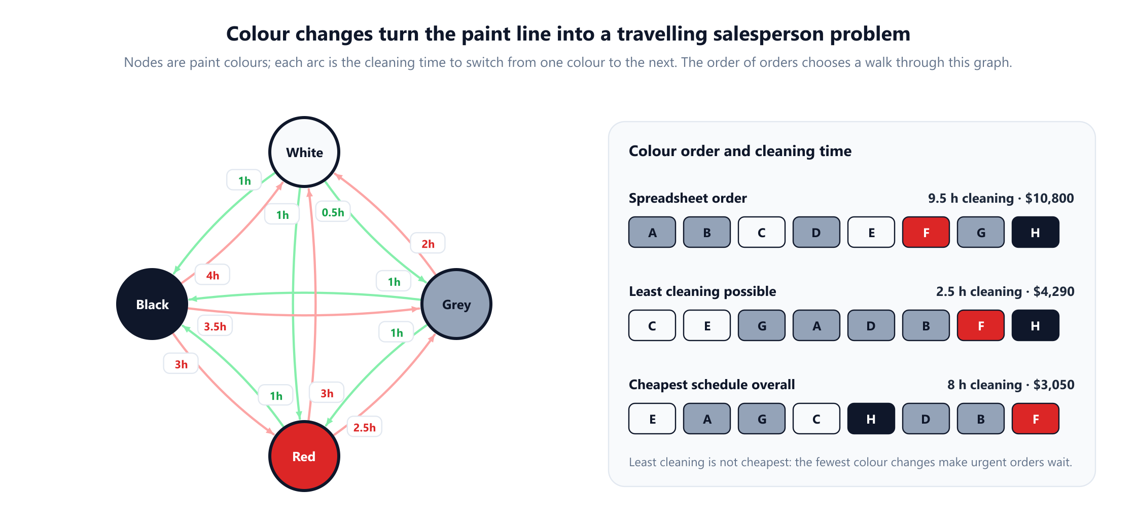
Picture the colours as nodes of a directed graph, with each arc weighted by its cleaning time. A sequence of orders is a walk through that graph, and minimising total cleaning time is finding the cheapest walk that visits the orders' colours in some order, which is the travelling salesperson problem. Because cleaning from black to white takes 4 hours and from white to black only 1, the distances are asymmetric, which makes it the asymmetric version. Allahverdi and colleagues' 2008 survey reviews the large literature on scheduling with setup times like these.
The spreadsheet order loses 9.5 hours to cleaning. Several sequences manage the least cleaning possible, only 2.5 hours, and even the cheapest of them, such as C, E, G, A, D, B, F, H with light colours first and black last, costs $4,290, because grouping colours makes urgent orders wait behind less urgent ones of the same colour. The cheapest schedule overall spends 8 hours cleaning. Minimising changeovers is a popular rule on the shop floor, and here it is the wrong objective.
7. Smarter heuristics: NEH and local search
NEH. The heuristic of Nawaz, Enscore and Ham (1983) sorts orders by total processing time, longest first, and inserts them one at a time into the position of the growing sequence that gives the lowest cost so far. In Ruiz and Maroto's 2005 comparison of flow shop heuristics it was the strongest constructive method for the makespan objective. Applied to this week's total cost, it gives $5,450: better than three of the four simple rules, worse than weighted shortest first. It was designed to finish early, and finishing early is not this problem's objective.
Local search. Starting from any sequence, try every swap of two orders and every move of one order to another position, apply the change that saves most, and repeat until nothing helps. From the earliest due date sequence it makes two moves, swapping G with E and then moving G to fifth place, reaching $3,500, and then stops. From that sequence no single swap or move saves money, although a sequence costing $3,050 exists. It is a local optimum.
From the spreadsheet order, the same local search takes five moves and reaches the optimum of $3,050. The outcome depends on where the search starts, which is why practical schedulers restart local search from several sequences or use metaheuristics, such as the tabu search of Nowicki and Smutnicki (1996) for job shops, that are allowed to accept worse moves temporarily to escape local optima.
8. The exact answer
With eight orders, all 40,320 sequences can be scheduled and priced in well under a second. The cheapest is E, A, G, C, H, D, B, F, and no other sequence ties with it.
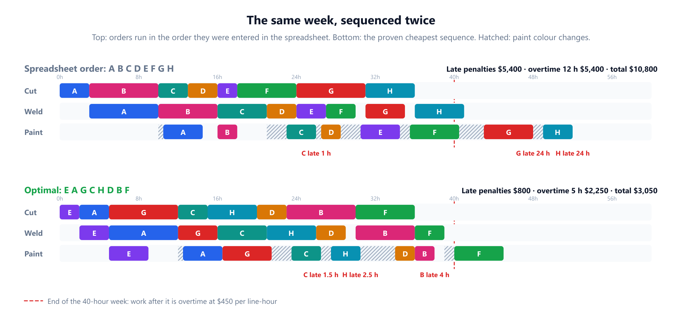
The optimum costs $3,050: three orders a little late, C by 1.5 hours, H by 2.5 and B by 4, for $800 of penalties, and 5 hours of overtime for $2,250. It is worth noticing what it does not do. It does not make every order on time, because that is impossible within this week, and it does not avoid overtime entirely. It trades small, cheap delays on low-penalty orders for the long, expensive delays the other sequences create.
| Method | Sequence | Finish | Late penalties | Overtime | Total | Above optimum |
|---|---|---|---|---|---|---|
| Spreadsheet order | A B C D E F G H | 52 h | $5,400 | $5,400 | $10,800 | +$7,750 |
| Shortest job first | D E C H A F B G | 49 h | $3,960 | $4,050 | $8,010 | +$4,960 |
| Earliest due date | G C A H B D E F | 53.5 h | $1,635 | $6,075 | $7,710 | +$4,660 |
| NEH insertion | E H C B G A D F | 47 h | $2,300 | $3,150 | $5,450 | +$2,400 |
| Weighted shortest first | E C D H A G B F | 45.5 h | $2,350 | $2,475 | $4,825 | +$1,775 |
| Earliest due date, then local search | E C A H G B D F | 45 h | $1,250 | $2,250 | $3,500 | +$450 |
| Proven optimum | E A G C H D B F | 45 h | $800 | $2,250 | $3,050 | 0 |
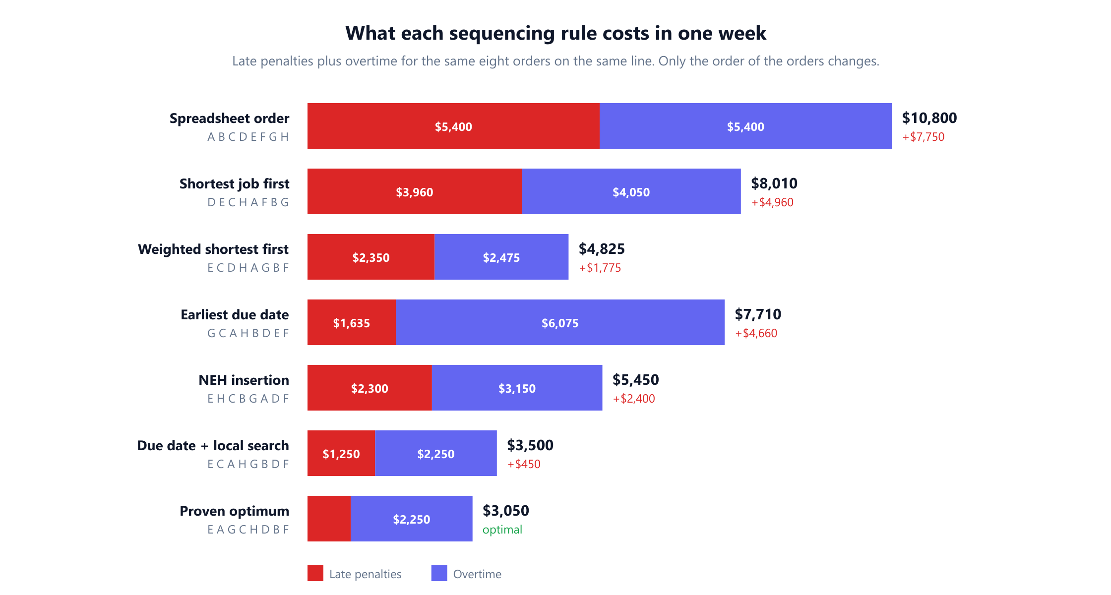
The gap between the spreadsheet and the optimum is $7,750 in one week: the spreadsheet's week costs more than three times as much as the optimal one. If a typical week looked like this one, that would be about $372,000 over 48 working weeks, which is the scale of saving that justifies a scheduling project.
Enumeration stops being practical quickly: 12 orders have almost 480 million sequences and 20 orders more than 2 × 10¹⁸. Real schedulers use branch and bound, constraint programming or the heuristics above, and the enumeration here serves the same purpose as a benchmark: it proves how far each method is from the best possible, which is information a planner never has in practice.
9. A rush order arrives
On Monday morning, before work starts, an important customer places a rush order R: 3 hours of cutting, 5 of welding and 2 of painting in black, due at hour 21, with a penalty of $200 per late hour. The planner has three options.
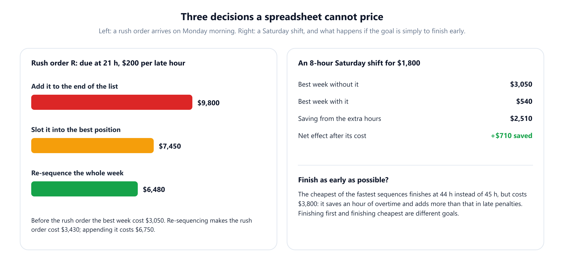
- Add it to the end of the list, the spreadsheet reflex. R finishes 27 hours late, $5,400 of penalty on its own, and the week costs $9,800.
- Slot it into the best position of the existing optimal sequence without moving anything else. The best slot is fifth, and the week costs $7,450.
- Re-sequence the whole week from scratch, checking all 9! = 362,880 sequences. The best is E, C, R, H, G, A, B, D, F, which delivers R on time and costs $6,480.
So accepting the rush order costs $3,430 if the week is re-planned properly, and $6,750 if it is simply appended. That number has two uses. It is the minimum rush surcharge that makes the order worth taking, and it is the value of being able to re-plan quickly: a planner with an optimiser saves $3,320 on this one decision compared with one who appends.
10. Is a Saturday shift worth it?
The optimal week still needs 5 hours of overtime. Suppose an 8-hour Saturday shift can be scheduled for a fixed $1,800, which extends the normal week to 48 hours before overtime starts.
Re-solving all 40,320 sequences with the longer week gives a best cost of $540, with no overtime and three small delays. The Saturday shift saves $2,510 in penalties and overtime against its $1,800 cost, a net saving of $710, so this week it is worth scheduling. Note that the best sequence changes when capacity changes: with Saturday available, the optimum starts with A and G rather than E. Capacity and sequence have to be decided together, which is precisely what the spreadsheet cannot do.
11. Finishing first is not finishing cheapest
Much of the scheduling literature, and many planning tools, minimise the makespan, the time the last order finishes. On this week the fastest possible finish is 44 hours, one hour earlier than the optimum, and several sequences reach it. The cheapest of them, such as E, A, G, C, F, H, D, B, costs $3,800, $750 more than the optimum: finishing an hour earlier saves $450 of overtime, and the order of work needed to do it adds $1,200 of late penalties. Finishing early is a proxy for good scheduling, and a poor one when customers have different due dates and penalties.
For two machines, the makespan problem has an elegant exact solution. Johnson's rule (1954) splits the orders into those faster on the first machine than the second, run first in increasing order of their first-machine time, and the rest, run last in decreasing order of their second-machine time. Applied to Cut and Weld alone, it gives the sequence E, A, C, D, H, B, G, F, finishing at 39 hours, and checking every sequence confirms that 39 hours is the minimum. Add the third machine and no such rule exists: Garey, Johnson and Sethi proved in 1976 that minimising makespan in a three-machine flow shop is NP-hard.
12. Job shops and the disjunctive graph
Many plants are not lines. In a job shop, each job has its own route through the machines: one order goes Cut, Weld, Paint, another Weld, Paint, Cut. Schedules can no longer be written as a single sequence, and the graph from section 4 needs one more idea, due to Roy and Sussmann (1964).
Draw a node for every operation and a solid arc along each job's route. Then, for every pair of operations that need the same machine, add a disjunctive pair of arcs, one in each direction, meaning "one of these must go first". A schedule is a choice of one direction for every pair. The choice is feasible exactly when the resulting directed graph has no cycle, and its makespan is the longest path through it.
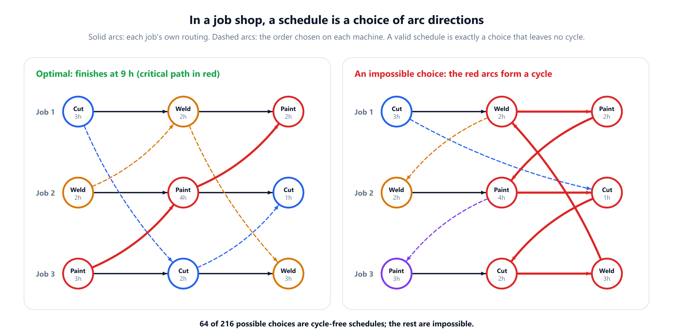
The small job shop in the figure has three jobs on three machines. Each machine can process its three operations in 3! = 6 orders, so there are 63 = 216 ways to orient the disjunctive arcs, and only 64 of them are acyclic. The other 152 describe schedules that cannot exist, where, for example, job 1's weld waits for job 3's weld, which waits for job 3's cut, which waits, around the cycle, for job 1's weld again.
Among the 64 valid schedules the best finishes at 9 hours, and it is provably optimal without further search: the three paint operations alone need 3 + 4 + 2 = 9 hours on one machine, so no schedule can finish sooner. Its critical path runs through exactly those three paint operations. The worst valid schedule takes 22 hours, which is the total processing time of all nine operations run one after another with no parallel work at all.
This graph is how serious job shop algorithms work. Balas's 1969 implicit enumeration branched on arc directions, the shifting bottleneck heuristic of Adams, Balas and Zawack (1988) orients one machine's arcs at a time, and tabu search methods move between schedules by reversing arcs on the critical path, because only those reversals can shorten the makespan.
13. What is easy, what is hard
| Problem | Method | Difficulty |
|---|---|---|
| Start and finish times for a given sequence | Longest paths in an acyclic graph | Linear time |
| Single machine, minimise the maximum lateness | Earliest due date (Jackson, 1955) | Polynomial |
| Single machine, minimise total weighted completion time | Weighted shortest processing time (Smith, 1956) | Polynomial |
| Two-machine flow shop, minimise makespan | Johnson's rule (1954) | Polynomial |
| Single machine, minimise total tardiness | Pseudo-polynomial dynamic programme (Lawler, 1977) | NP-hard (Du and Leung, 1990) |
| Three-machine flow shop, minimise makespan | Branch and bound, NEH, local search | NP-hard (Garey, Johnson and Sethi, 1976) |
| Sequence-dependent setup times | Contains the travelling salesperson problem | NP-hard |
| Job shop, minimise makespan | Disjunctive graph, shifting bottleneck, tabu search | NP-hard |
Lenstra, Rinnooy Kan and Brucker's 1977 classification maps hundreds of such variants, using the notation Graham, Lawler, Lenstra and Rinnooy Kan formalised in 1979. The practical reading is the same as for other planning problems: evaluating a schedule is easy, finding the best one is hard, and good methods combine fast evaluation with clever search. Taillard's 1993 benchmark instances are still how new flow shop and job shop methods are compared.
14. What the model leaves out
- Release dates. Materials arrive during the week, so some orders cannot start at hour zero.
- Parallel machines. Real lines often have two welders or several paint booths, which adds an assignment decision to the sequence.
- Breakdowns and uncertain times. Processing times vary and machines fail, so schedules need slack, and re-scheduling policy matters as much as the original plan.
- Labour and skills. Operators, not only machines, can be the constraint, which links production scheduling to employee shift scheduling.
- Batching and lot sizing. Orders are often split or combined, and how many to run together is its own optimisation.
- Material planning. Components must be available when an order starts, which is the job of material requirements planning upstream of the schedule.
None of these changes the core picture: operations as nodes, precedence and machine order as arcs, and cost computed from longest paths. Constraint programming solvers handle most of them directly, which is one reason they have become popular for industrial scheduling.
15. From spreadsheet to optimisation
Start with the data you already have. Routings and standard times usually exist in the ERP or MES system; due dates and customer priorities exist in sales; setup times exist in the heads of experienced operators and should be written down as a matrix. Checking standard times against actual times is usually the first surprise of a scheduling project.
Price the current way of working. Take last month's actual sequences and compute their late penalties, overtime and changeover hours with the same model. That baseline shows what is at stake, and it tests whether the model's costs match what finance sees.
Choose tools that fit the plant. Google OR-Tools' CP-SAT solver has interval variables designed for scheduling; mixed integer programming solvers such as HiGHS and Gurobi work well for smaller or highly structured problems; and advanced planning and scheduling systems package the same methods with shop floor integration. The Theory of Constraints, popularised by Goldratt and Cox's 1984 novel The Goal, is a useful complement: it keeps attention on the bottleneck, which is the critical path in graph terms.
Re-plan on a rhythm, and involve the planners. Most plants re-sequence daily or per shift, freezing the next few hours so the floor is not disrupted. Planners know about urgent calls and fragile tooling that no system records, and the most effective deployments let them adjust the optimiser's plan and see the cost of each adjustment before they make it.
16. Mistakes that quietly cost money
- Running orders in the order they arrived. The spreadsheet order cost $7,750 more than the optimum, and was worse than the median of all possible sequences.
- Treating one rule as the answer. Earliest due date minimises the worst lateness, not the total cost, and here it ran the most overtime of any method.
- Minimising changeovers for their own sake. The least-cleaning sequence cost $4,290 against the optimum's $3,050.
- Minimising makespan when customers have due dates. Finishing an hour earlier cost $750 more.
- Appending rush orders. Adding the rush order to the end cost $3,320 more than re-sequencing the week.
- Deciding capacity separately from sequence. The Saturday shift paid for itself only because the sequence was re-optimised around it.
- Guessing the bottleneck. The finish time is a longest path, and with ties there can be more than one. Compute it.
- Trusting a heuristic without a benchmark. Local search from the due date sequence stopped $450 above the optimum and gave no sign of it.
17. Frequently asked questions
What is production scheduling?
+
It is deciding when each order runs on each machine, in what sequence, so that orders are delivered on time, machines and people are used within their capacity, and costs such as overtime, late penalties and changeovers are as low as possible. In operations research it is studied as machine scheduling, with standard models for single machines, flow shops where every order follows the same route, and job shops where routes differ.
Why is spreadsheet production scheduling not good enough?
+
A spreadsheet lists orders but cannot search the enormous number of possible sequences or price the interactions between due dates, penalties, machine queues and changeovers. In this article's example, running eight orders in the order they were entered cost $10,800 in a week, while the best sequence of the same orders cost $3,050. Spreadsheets also make it hard to re-plan quickly when a rush order arrives or capacity changes.
Which dispatching rule is best: EDD, SPT or FIFO?
+
Each is optimal for a different simplified problem. Earliest due date minimises maximum lateness on a single machine, shortest processing time minimises average completion time, and weighted shortest processing time minimises total weighted completion time. None is optimal for a multi-machine line with due dates, different penalties, overtime and setups. In the example, weighted shortest first was the best simple rule but still $1,775 above the optimum.
How does graph theory help with production scheduling?
+
For a fixed sequence, operations and their precedence form a directed acyclic graph, and the finish time is the longest path through it, whose operations form the critical path. In a job shop, the disjunctive graph of Roy and Sussmann represents each machine's possible orders as pairs of arcs, and a schedule is feasible exactly when the chosen directions create no cycle. Sequence-dependent setups make the sequencing problem a travelling salesperson problem.
What is Johnson's rule?
+
A 1954 algorithm that minimises makespan when every job passes through the same two machines. Jobs whose first-machine time is at most their second-machine time go first, in increasing order of first-machine time; the others go last, in decreasing order of second-machine time. It is provably optimal for two machines, but no such rule exists for three or more, where minimising makespan is NP-hard.
How should a rush order be scheduled?
+
Re-sequence the remaining work rather than appending the order or squeezing it into one slot. In the example, re-sequencing the week delivered the rush order on time and made it cost $3,430 in extra penalties and overtime, while appending it to the end cost $6,750. The re-planned cost is also the minimum surcharge that makes the rush order worth accepting.
What software is used for production scheduling optimization?
+
Google OR-Tools provides the CP-SAT constraint programming solver with interval variables built for scheduling, mixed integer programming solvers such as HiGHS and Gurobi handle smaller or structured models, and advanced planning and scheduling systems add integration with ERP and shop floor data. Many plants start by rebuilding their spreadsheet logic in a model, pricing their current schedules as a baseline, and then optimising daily with a frozen window for the next few hours.
18. References
The foundational papers, surveys and books behind the methods in this article, in chronological order.
- Johnson, S. M. (1954). “Optimal two- and three-stage production schedules with setup times included.” Naval Research Logistics Quarterly, 1(1), 61–68.
- Jackson, J. R. (1955). Scheduling a Production Line to Minimize Maximum Tardiness. Research Report 43, Management Science Research Project, University of California, Los Angeles.
- Smith, W. E. (1956). “Various optimizers for single-stage production.” Naval Research Logistics Quarterly, 3(1–2), 59–66.
- Roy, B. and Sussmann, B. (1964). Les problèmes d'ordonnancement avec contraintes disjonctives. Note DS no. 9 bis, SEMA, Paris.
- Balas, E. (1969). “Machine sequencing via disjunctive graphs: an implicit enumeration algorithm.” Operations Research, 17(6), 941–957.
- Garey, M. R., Johnson, D. S. and Sethi, R. (1976). “The complexity of flowshop and jobshop scheduling.” Mathematics of Operations Research, 1(2), 117–129.
- Lawler, E. L. (1977). “A ‘pseudopolynomial’ algorithm for sequencing jobs to minimize total tardiness.” Annals of Discrete Mathematics, 1, 331–342.
- Lenstra, J. K., Rinnooy Kan, A. H. G. and Brucker, P. (1977). “Complexity of machine scheduling problems.” Annals of Discrete Mathematics, 1, 343–362.
- Graham, R. L., Lawler, E. L., Lenstra, J. K. and Rinnooy Kan, A. H. G. (1979). “Optimization and approximation in deterministic sequencing and scheduling: a survey.” Annals of Discrete Mathematics, 5, 287–326.
- Nawaz, M., Enscore, E. E. and Ham, I. (1983). “A heuristic algorithm for the m-machine, n-job flow-shop sequencing problem.” Omega, 11(1), 91–95.
- Goldratt, E. M. and Cox, J. (1984). The Goal: A Process of Ongoing Improvement. Great Barrington: North River Press.
- Adams, J., Balas, E. and Zawack, D. (1988). “The shifting bottleneck procedure for job shop scheduling.” Management Science, 34(3), 391–401.
- Du, J. and Leung, J. Y.-T. (1990). “Minimizing total tardiness on one machine is NP-hard.” Mathematics of Operations Research, 15(3), 483–495.
- Taillard, E. (1993). “Benchmarks for basic scheduling problems.” European Journal of Operational Research, 64(2), 278–285.
- Nowicki, E. and Smutnicki, C. (1996). “A fast taboo search algorithm for the job shop problem.” Management Science, 42(6), 797–813.
- Ruiz, R. and Maroto, C. (2005). “A comprehensive review and evaluation of permutation flowshop heuristics.” European Journal of Operational Research, 165(2), 479–494.
- Allahverdi, A., Ng, C. T., Cheng, T. C. E. and Kovalyov, M. Y. (2008). “A survey of scheduling problems with setup times or costs.” European Journal of Operational Research, 187(3), 985–1032.
- Pinedo, M. L. (2016). Scheduling: Theory, Algorithms, and Systems, 5th edition. Cham: Springer.