Graph Theory in Biology

Mohammed Islam Hadjoudj

Expert Operations Research Engineer

1. Why biology is full of graphs

Biology spent most of its history making lists. A list of genes, a list of enzymes, a list of the species in a lake. The lists got long and then they got complete, and completing them revealed something uncomfortable: knowing every part of a system tells you remarkably little about what the system does. The human genome was finished in 2003 and the number of protein-coding genes turned out to be around 20,000, not far off the count in a nematode worm with 302 neurons. The parts list was never going to be the explanation.

What separates a human from a worm, and a healthy cell from a cancerous one, is not which components exist but which components interact with which. That sentence is a definition of a graph. A graph is a set of things together with a set of connections between them, and nothing else. The moment you write down which proteins bind to which, or which gene switches on which, or which species eats which, you have stopped making a list and started drawing a graph, whether or not you use the word.

This is not a metaphor and it is not a presentation style. It matters because graphs arrive with two centuries of mathematics attached. Once a biological question is phrased as a graph question, a large body of theorems and algorithms becomes available at once, and problems that look like they need new biology turn out to need an existing algorithm instead. Genome assembly, the process that turns hundreds of millions of short DNA fragments into a chromosome, is a walk that uses every edge of a graph exactly once. Euler settled that problem in 1736 for the bridges of a Prussian city, and it is the same problem.

The habit is older than most people assume. The word graph in this technical sense was coined by the mathematician James Joseph Sylvester in 1878, by analogy with chemical structure diagrams: molecules drawn as atoms joined by bonds. Chemistry gave graph theory part of its vocabulary, and a century later molecular biology gave it some of its largest data sets.

This guide works through six biological systems: a protein interaction network, a gene regulatory network, a genome being assembled from reads, a pair of sequences being aligned, a set of species placed on an evolutionary tree, and a food web losing species one at a time. Each is kept small enough to check by hand and solved with a named algorithm. Every number here came out of code that was run, and each result was recomputed by a second, different method before it was written down.

2. Four graphs, four different questions

Before building anything it is worth being precise about what kind of graph each biological system produces, because the kind decides which questions are even askable. Four distinctions do almost all of the work.

Directed or undirected. If two proteins bind, the relationship is symmetric: "A binds B" and "B binds A" are the same fact, so protein interaction networks are undirected. If a transcription factor switches on a gene, the relationship runs one way, so gene regulatory networks are directed. This is not bookkeeping. Undirected graphs have connected components; directed graphs have reachability, cycles and feedback, and feedback is the substance of regulation. Asking whether a gene network contains a cycle is asking whether it contains a feedback loop, and the answer changes the biology.

Weighted or unweighted. A food web edge can simply exist, or it can carry the biomass flowing along it. Sequence similarity graphs carry a score on every edge. Weights let you ask for the best route rather than merely a route, which is what turns alignment into a shortest path problem in section 8.

Static or dynamic. Almost every network in this article is drawn as though it were fixed. Real cells are not. An interaction that exists in a liver cell may not exist in a neuron, and interactions appear and vanish across the cell cycle. Treating a time-averaged aggregate as though all of its edges were simultaneously present is the most common modelling error in this field, and section 13 comes back to it.

Bipartite or not. Some biological data has two kinds of vertex with edges only between the kinds: drugs and their targets, hosts and their parasites, genes and the diseases they are associated with. Bipartite graphs bring their own algorithms, matching above all, which is how drug repurposing screens are often framed.

Get these four right and the rest follows. Get them wrong and you will compute a number that is meaningless in a way no software will warn you about.

3. Protein networks: hubs, bridges and betweenness

A protein interaction network, usually shortened to PPI network, has one vertex per protein and an undirected edge wherever two proteins physically bind. Large-scale versions are built by yeast two-hybrid screens or by affinity purification followed by mass spectrometry, and the published networks for yeast and human run to tens of thousands of edges. Rather than gesture at something enormous, we will use a small one: twelve proteins and eighteen interactions, small enough that every claim below can be checked by counting.

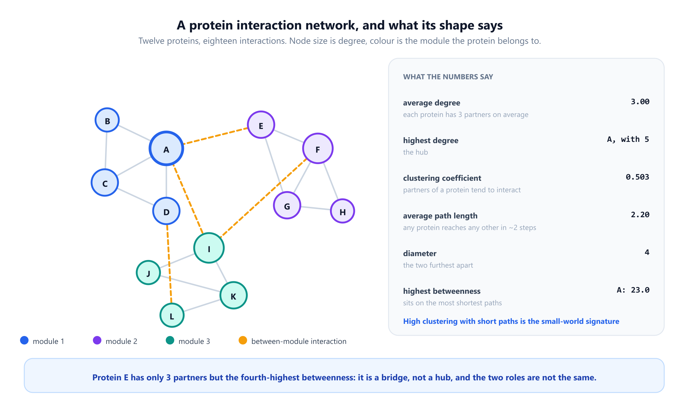
The first thing to measure is degree, the number of partners a protein has. Here the degrees run A:5, then F and I with 4, then a group of five with 3, then a tail of four with 2, averaging 3.0. In real PPI networks this distribution is far more uneven: most proteins have a handful of partners and a small minority have hundreds. Networks with that shape are called scale-free, a term Barabasi and Oltvai popularised in their 2004 review, and the high-degree minority are the hubs.

Hubs matter for a reason that was established experimentally rather than argued theoretically. In 2001 Jeong, Mason, Barabasi and Oltvai compared the yeast PPI network against the yeast deletion library, in which every gene has been knocked out in turn and the resulting cell scored viable or dead. Proteins with more interaction partners were substantially more likely to be essential. The paper is called Lethality and centrality in protein networks, and the correlation it reported is why degree became the first thing anyone computes on a biological network.

Degree is not the only kind of importance, and this is where a small example earns its place. Consider protein E. It has three partners and on any list sorted by degree it is unremarkable. Now compute betweenness centrality, which counts, over every pair of proteins, what fraction of the shortest paths between them passes through a given vertex. Freeman introduced the measure in 1977 for social networks. On this graph the betweenness ranking is A at 23.0, I at 19.8, F at 12.2, and then E at 9.2, ahead of several proteins with more partners than it has.

E scores highly because of where it sits, not how many neighbours it has. It is the entry point of the second module, so traffic between the first module and the second has to pass through it. In network terms E is a bridge rather than a hub, and the distinction has a biological reading: bridge proteins are candidates for cross-talk between pathways, and removing one does not delete a function so much as disconnect two functions from each other. A ranking by degree alone would never surface it.

Two further numbers describe the whole graph rather than any single vertex. The average shortest path length is 2.197 and the diameter, the longest of all shortest paths, is 4: any protein reaches any other in at most four steps. Real PPI networks behave the same way at vastly larger scale, with thousands of proteins and a characteristic path length around 5. This is the small-world property that Watts and Strogatz formalised in 1998, and inside a cell it has a blunt consequence. A perturbation anywhere is a few steps from everywhere, which is a large part of why a drug aimed at one protein so reliably produces effects nobody designed.

4. Robust to accidents, fragile to attack

The most cited result in network biology is not about any particular protein. It is about what happens when you start deleting them, and it was published by Albert, Jeong and Barabasi in Nature in 2000 under the title Error and attack tolerance of complex networks.

The experiment is easy to state. Take a network, remove vertices, and after each removal measure the size of the largest surviving component. Do it twice: once removing vertices uniformly at random, which models accidents and mutation, and once removing them in descending order of degree, which models a deliberate attack. Then compare the curves.

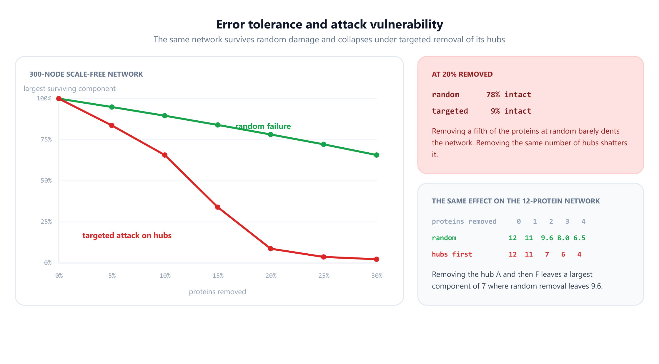
On a 300-vertex scale-free network grown by preferential attachment, removing 20% of the vertices at random leaves 78% of the network still connected in one piece. Removing the 20% with the highest degree leaves 9%. The network that shrugged off the first attack was destroyed by the second, and the only difference between them was which vertices got chosen.

The twelve-protein network shows the same asymmetry at a scale you can verify by hand. Removing proteins at random, averaged over every possible choice, leaves largest components of 12, 11, 9.55, 7.96 and 6.46 as the number of removals goes from zero to four. Removing hubs in descending degree order, which here means A, then F, then I, then C, leaves 12, 11, 7, 6 and 4. Two well-chosen deletions cost more than four random ones.

The explanation is the degree distribution. In a scale-free network the overwhelming majority of vertices have low degree, so a random deletion almost certainly hits a peripheral vertex whose loss disconnects nobody. The rare hubs hold everything together, and deleting one removes many edges at once. Robustness against random damage and fragility against targeted damage are not two properties in tension. They are one property viewed from two directions.

The biological readings run both ways. On the fragile side, this is why hub proteins are enriched for essentiality, and why oncology has spent two decades trying to identify the hubs a tumour depends on. On the robust side, it is why organisms tolerate an enormous load of random mutation with no visible consequence, and why single-gene knockouts so often produce no phenotype at all. That last observation frustrated a generation of geneticists: most genes are not load-bearing, and the ones that are can be picked out by their position in the graph.

5. Modules, and why clustering means function

Look again at the twelve-protein network and you can see three groups by eye. Proteins A to D are densely tied to each other, E to H form a second cluster, I to L a third, and only four edges cross between groups. That visual impression has a number behind it.

The clustering coefficient of a vertex asks a specific question: of all the pairs of my neighbours, what fraction are themselves connected? If a protein has four partners there are six pairs among them, and the coefficient is the fraction of those six pairs that bind each other. Averaged over all twelve proteins this network scores 0.503, meaning roughly half of all the triangles that could close do close. A random graph with the same number of vertices and edges scores about 0.23. Real PPI networks are similarly clustered, and so are metabolic networks, neural networks and food webs.

High clustering is what makes the word module meaningful. Proteins that all bind each other tend to be doing one job together: they form a complex, or sit in one pathway, or are recruited to the same place at the same time. This is the most useful inference in applied network biology, because it lets you annotate an unknown protein from its neighbours. If a protein of unknown function sits in a cluster whose other members all handle DNA repair, DNA repair is the hypothesis to test first. Whole pipelines rest on that idea, and they are community detection algorithms with biological names attached.

One caution belongs here. A module found by an algorithm is a hypothesis, not a discovery. The algorithm partitions whatever you give it, and it will return modules from random data just as happily.

6. Gene regulation: network motifs

Gene regulatory networks are directed. An arc from gene X to gene Y means the protein X produces binds the promoter of Y and changes how much of Y gets made. Because the arcs have direction, the interesting structures are patterns of flow rather than dense neighbourhoods, and in 2002 two papers from Uri Alon's group changed how people read them.

The idea is this. Take a small subgraph, say three genes wired in a particular pattern, and count how often it occurs in the real network. That count alone means nothing, because some patterns are common purely as a consequence of how many arcs each gene has. So generate many randomised networks with exactly the same degrees, by repeatedly swapping the endpoints of pairs of arcs, and count the pattern in each. If the real count sits far out in the tail of that distribution, the pattern is a network motif: it occurs more often than the degrees alone can explain, which is evidence that selection put it there.

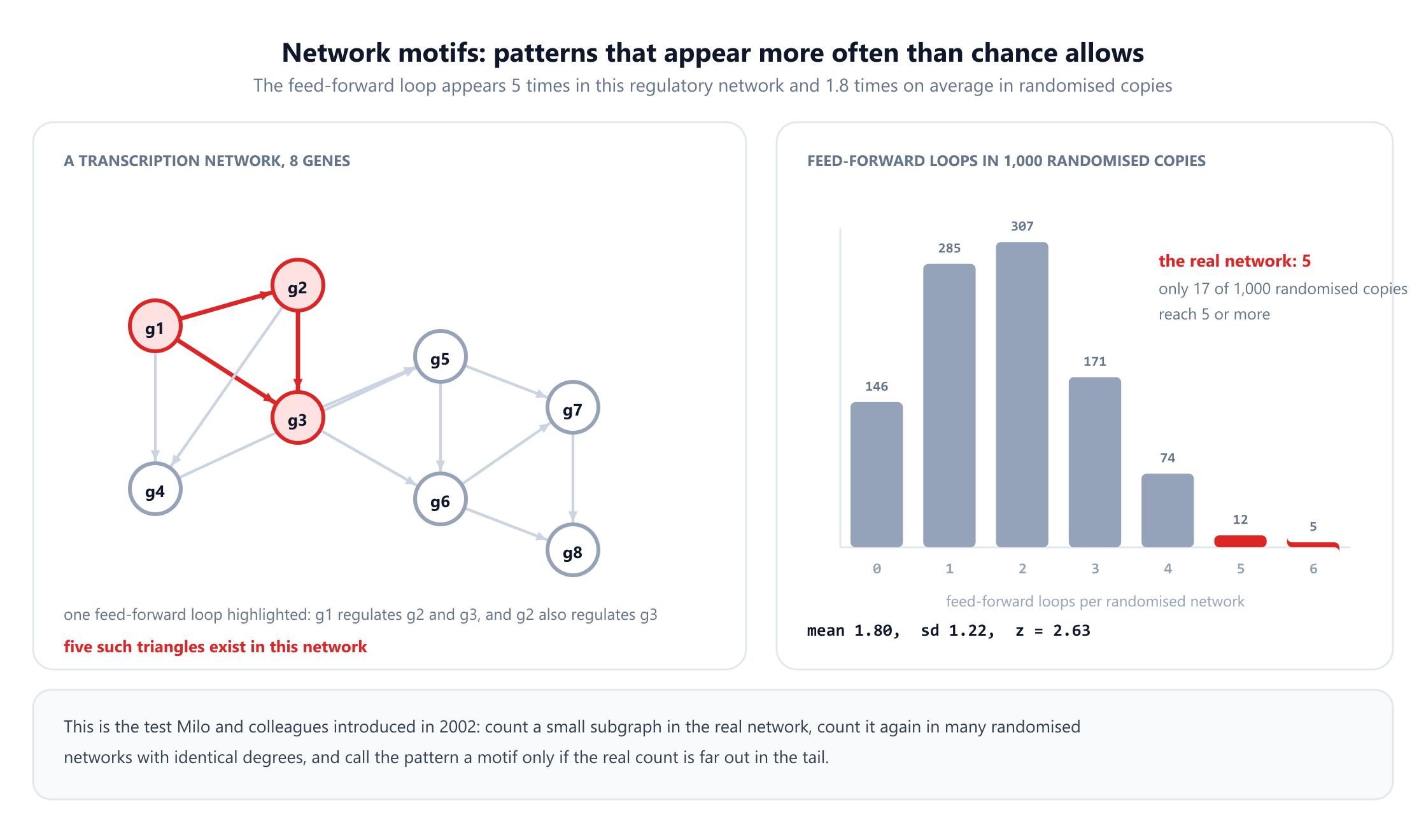
The pattern in the figure is the feed-forward loop: gene X regulates Y, X also regulates Z directly, and Y regulates Z as well. In the eight-gene network here it occurs five times. Across 1,000 degree-preserving randomisations the average count was 1.80 with a standard deviation of 1.22, giving a z-score of 2.63, and only 17 of the 1,000 randomised networks contained five or more. On a network this small that is suggestive rather than conclusive; in the real E. coli transcription network Shen-Orr, Milo and Alon found the same pattern with z-scores in the tens, which is not a borderline result.

What makes the feed-forward loop worth caring about is that its function can be derived rather than guessed. In the coherent version, where X activates both Y and Z and Y also activates Z, gene Z only switches on once both X and Y are present. Since Y takes time to accumulate after X appears, Z ignores brief pulses of X and responds only to sustained signals. The motif is a persistence detector, a noise filter built out of three genes. Change the signs and you get a pulse generator or an accelerated response instead. The wiring is the mechanism.

Milo and colleagues found that different kinds of network are characterised by different motifs: transcription networks are rich in feed-forward loops, neural networks in a different set, food webs in another again. They argued that motifs are the elementary circuits from which the network is built, and the framing stuck, both because the statistics are checkable and because the circuits do something.

One methodological point generalises well beyond biology. The randomisation must preserve degrees. Compare against an ordinary random graph and almost everything looks like a motif, since real networks have hubs and random ones do not, and the hubs alone generate a surplus of every three-node pattern. Getting the null model wrong is the standard way this analysis fails.

7. Genome assembly: walking every edge once

Sequencing machines cannot read a chromosome. They read short fragments, from around 100 bases on a short-read instrument up to tens of thousands on a long-read one, sampled at random positions from many copies of the genome. A human genome arrives as hundreds of millions of these fragments with no record of where any of them came from. Assembly is the problem of putting them back together, and the modern solution is a graph.

The construction is due to Pevzner, Tang and Waterman in 2001, and it is elegant enough to state in two sentences. Chop every read into overlapping substrings of length k, called k-mers. Then build a graph in which each k-mer is an edge, running from the vertex spelled by its first k-1 letters to the vertex spelled by its last k-1 letters. Reconstructing the sequence now means finding a walk that uses every edge exactly once, which is an Eulerian path.

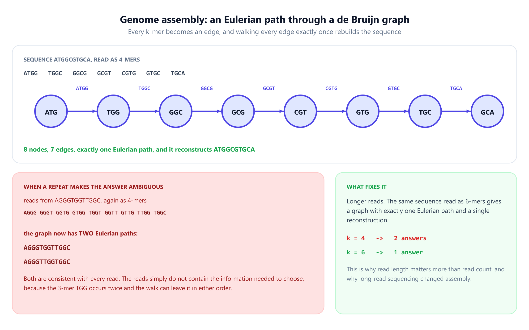
Take the sequence ATGGCGTGCA and read it as 4-mers. That gives seven k-mers, a graph with 8 vertices and 7 edges, and exactly one Eulerian path, which spells the original sequence back out. Assembly succeeded, and it succeeded because the graph had a unique answer.

Now take AGGGTGGTTGGC, again as 4-mers. The graph has two Eulerian paths, spelling AGGGTGGTTGGC and AGGGTTGGTGGC. Both are consistent with every read that was observed. This is not a failure of the algorithm, and no better algorithm can fix it: the 3-mer TGG occurs twice, the walk arrives at that vertex more than once, and the reads carry no information about which way to leave it the first time. The ambiguity is in the data.

What resolves it is longer reads. Reading the same sequence as 6-mers produces a graph with exactly one Eulerian path and a single reconstruction. This is the reason the sequencing industry has spent fifteen years chasing read length rather than read count, and the reason the human genome was only declared complete, gap to telomere, in 2022, more than twenty years after the first draft. The missing pieces were repeats, and repeats are precisely the structures that make an Eulerian walk ambiguous.

There is a lovely piece of algorithmic history here. Finding an Eulerian path is easy: linear time, with an existence condition known since Euler. The natural-looking alternative, building a graph in which every read is a vertex and joining reads that overlap, requires a walk visiting every vertex once, which is a Hamiltonian path and NP-complete. Two formulations of one biological task, one tractable and one hopeless, separated only by the decision to make the reads edges instead of vertices.

8. Sequence alignment is a shortest path

Comparing two sequences is the most-run computation in biology. Every BLAST query does it, every read mapper does it, and every claim that two genes are homologous rests on it. The standard algorithm is Needleman and Wunsch's, published in 1970 and taught everywhere as dynamic programming over a matrix. It is worth seeing that the matrix is a graph.

Build a grid with one vertex for each pair of positions (i, j), meaning "the first i letters of sequence one have been aligned against the first j letters of sequence two". From each vertex draw three arcs: right, for a letter of sequence two against a gap; down, for a letter of sequence one against a gap; and diagonal, for aligning the two letters. Give each arc a cost, zero for a diagonal that matches and one otherwise. The best alignment is now the cheapest path from the top-left corner to the bottom-right, and any shortest path algorithm finds it.

Aligning GATTACA against GCATGCU builds a grid graph with 64 vertices and 161 arcs. Needleman-Wunsch returns an edit distance of 4. A shortest path search over that graph, with no dynamic programming table anywhere, returns 4 as well. They agree because they are the same computation: the grid is acyclic, so filling the cells in order is exactly relaxing the arcs in topological order.

Seeing it as a graph is not a party trick. It explains why Smith and Waterman's 1981 local alignment algorithm works: allowing a path to start fresh anywhere is adding a zero-cost arc from the source to every vertex. It explains affine gap penalties, which need three layers of grid rather than one because the state must remember whether a gap is already open. And it explains why alignment costs the product of the two sequence lengths, since that is the size of the graph, which is why fast aligners avoid building most of it.

9. Phylogenetics: one tree out of astronomically many

A phylogenetic tree is a graph with no cycles: leaves are the species you observed, internal vertices are ancestors you did not, and edge lengths measure evolutionary divergence. Reconstructing one from present-day sequences is the central inference problem of evolutionary biology, and its difficulty is a counting problem before it is anything else.

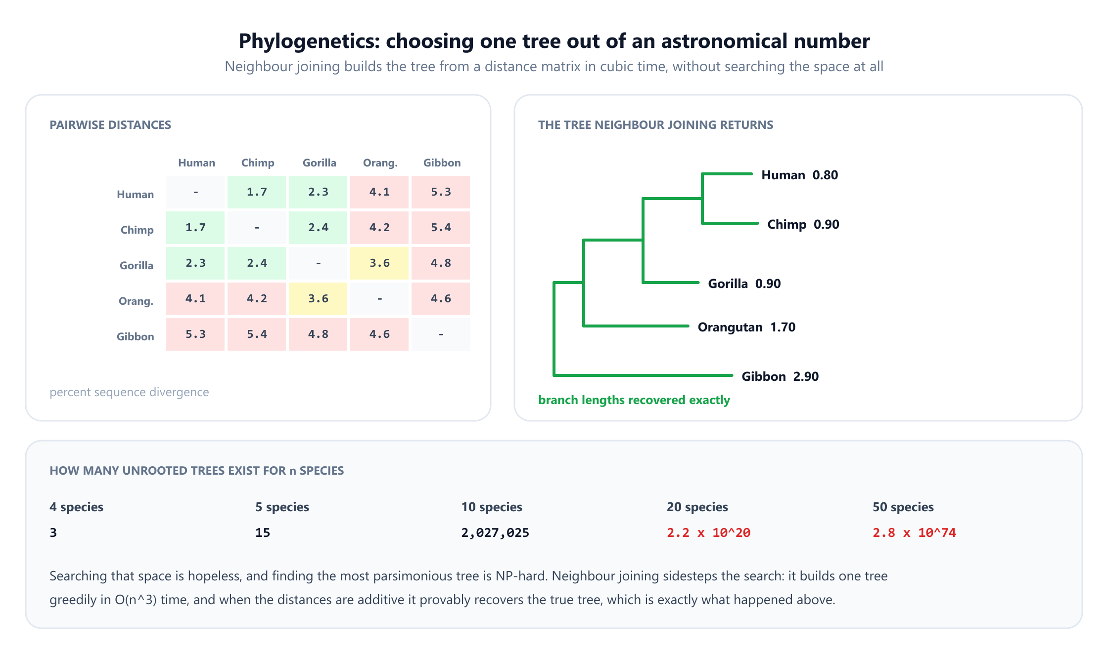
The number of distinct unrooted binary trees on n species, tabulated by Felsenstein in 1978, is the double factorial (2n-5)!!, and it detonates. Four species give 3 trees. Five give 15. Ten give 2,027,025. Twenty give about 2.2 x 10²⁰. Fifty species give roughly 2.8 x 10⁷⁴, which is more trees than there are atoms in the observable universe by a wide margin. Every one of those is a candidate answer, and phylogenetic studies routinely involve hundreds of taxa.

Exhaustive search is therefore not merely slow, it is permanently impossible, and the situation is worse than that: finding the most parsimonious tree, the one requiring the fewest evolutionary changes, was later proved NP-hard, and maximum likelihood tree search is no better.

Saitou and Nei's neighbour joining, published in 1987 and among the most cited papers in all of biology, sidesteps the search entirely. It takes a matrix of pairwise distances, repeatedly joins the pair of taxa that a specific criterion identifies as neighbours, and collapses them into one node, until a tree remains. It never enumerates alternatives, and it runs in cubic time.

On the five-primate distance matrix in the figure it joins orangutan with gibbon first, then human with chimp, then gorilla with the orangutan and gibbon group, and it recovers every branch length exactly. That exactness is not luck. When the distances are additive, meaning they came from some tree in the first place, neighbour joining provably returns that tree. Real distances estimated from real sequences are only approximately additive, which is why real phylogenetics uses neighbour joining to produce a fast starting tree and then refines it under a likelihood model, and why the same data set can support different published trees.

10. Food webs and extinction cascades

Move from inside the cell to a whole ecosystem and the mathematics does not change. A food web is a directed graph: one vertex per species, and an arc from prey to predator wherever the second eats the first. Species with no prey are basal, meaning plants, algae or detritus, and everything else ultimately depends on them.

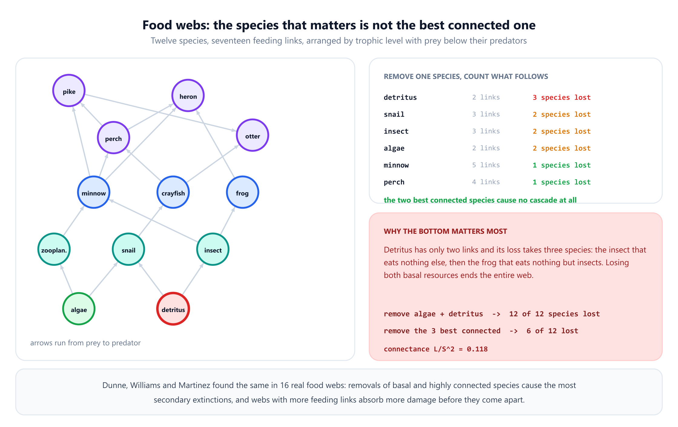
The model here has twelve species and seventeen feeding links, with algae and detritus at the base and an otter, a heron and a pike at the top. The first thing the graph gives you is trophic level, computed as one plus the average level of everything a species eats. Basal species sit at 1.00, herbivores at 2.00, and the top predators land on fractional values: the pike at 4.50, the otter at 4.75, the heron at 4.33. Fractional levels are not an artefact. They are the honest answer for an omnivore that eats at several levels at once.

The question that matters for conservation is what happens after a species is lost. Delete a vertex, then delete any species left with nothing to eat, then repeat until the web settles. Those follow-on losses are secondary extinctions, and they are the reason ecosystems collapse faster than the direct pressure on them would suggest.

The results on this web are counterintuitive in a specific and useful way. The minnow is the best connected species with five feeding links. Remove it and nothing else dies: everything that ate the minnow eats something else too. Remove the heron or the otter, both top predators, and again nothing follows. Now remove detritus, which has only two links and is not a species anybody campaigns to protect. Three species disappear in total: the detritus itself, then the insect that eats nothing else, then the frog that eats nothing but insects. A vertex with two edges caused more damage than a vertex with five.

The pattern generalises. Basal species are load-bearing because everything above them depends on them, while a highly connected consumer sits in a part of the graph that offers substitutes. Removing both basal species, algae and detritus, costs all twelve species. Removing the three best connected, minnow, perch and snail, costs six. Twice the damage from the less impressive-looking intervention.

Dunne, Williams and Martinez reported exactly this in 2002 across sixteen real food webs, and added a second finding worth carrying away: robustness increases with connectance, the number of links divided by the square of the number of species. Webs with more feeding links absorb more damage before they fragment, because more species have alternatives. The web modelled here has a connectance of 0.118, squarely in the range reported for real webs.

The practical lesson is that conservation triage based on charisma, size or even link count measures the wrong quantity. The species whose loss propagates is found by simulating the removal on the graph, and the answer is regularly something small and unloved.

11. Connectomes and epidemics

Two more areas deserve mention, because both reuse machinery already introduced.

Connectomes. A nervous system is a directed, weighted graph of neurons joined by synapses. The first complete one was published by White, Southgate, Thomson and Brenner in 1986: the nematode C. elegans, 302 neurons and around 7,000 connections, reconstructed by hand from electron micrographs over more than a decade. Human work operates at coarser resolution, with vertices as brain regions and edges as fibre bundles or correlated activity, but the analysis is the one from section 3: degree, clustering, path length, modules, hubs.

Bullmore and Sporns set out the programme in 2009, and the recurring finding is that brains are small-world and modular, with a densely interconnected core of high-degree regions, the "rich club", carrying a disproportionate share of long-distance traffic. Several psychiatric and neurological conditions show up as altered graph statistics. Those are correlations across groups, not diagnostics for individuals, and it is worth knowing that a functional connectome depends heavily on a correlation threshold chosen by the analyst, and that the statistics move when the threshold moves.

Epidemics. Disease spreads across a contact graph, and its structure determines the outcome as much as the pathogen does. Pastor-Satorras and Vespignani proved a startling result in 2001: on a network with a scale-free degree distribution and unbounded variance, the classical epidemic threshold vanishes. In the well-mixed models taught in textbooks an infection with a low enough transmission rate dies out; on such a network it does not, because the hubs keep it alive. That reframed vaccination strategy, since immunising the high-degree individuals, or even acquaintances of randomly chosen individuals, who are high-degree more often than chance, beats immunising at random with the same number of doses.

The same mathematics reappears in cell biology as signal propagation and in computer security as malware spread. The graph does not care what the vertices represent.

12. What is easy, what is hard

Framing a biological question as a graph question does not make it solvable. It makes the difficulty visible, which is more useful, and the boundary falls in surprising places.

Easy, meaning polynomial time and routine at scale. Degree, clustering coefficients and connected components are effectively free. Shortest paths, and therefore alignment, are cheap. Betweenness centrality on a sparse graph runs in time proportional to the product of the vertex and edge counts thanks to Brandes' algorithm. Eulerian paths are linear, spanning trees and flows are polynomial, and neighbour joining is cubic. Everything solved in this article is in this category, and all of it scales to graphs with millions of edges on a laptop.

Hard, meaning NP-hard with no polynomial algorithm expected. Finding the most parsimonious phylogenetic tree. Finding the largest set of species that all interact, which is maximum clique. Deciding whether one network is a subgraph of another, which underlies motif search on larger patterns. Finding a Hamiltonian path, the reason the overlap formulation of assembly was abandoned. Optimal graph partitioning, in its exact form.

Two observations make the boundary less discouraging than it sounds. First, hard problems in biology are usually attacked with heuristics that work well on the instances that actually arise: phylogenetics hill-climbs from a neighbour-joining start, and motif finders enumerate cleverly, which is fine for three- and four-vertex patterns. Second, the difference between the tractable and intractable formulations of one biological task is often just a modelling choice, as the k-mers-as-edges decision in assembly shows. Recognising which side of the line you are on before writing code is most of the benefit.

13. Modelling mistakes

Five errors account for most of the wrong conclusions drawn from biological networks. None of them is exotic and all of them are still in print.

Treating an aggregate as a snapshot. A published PPI network is the union of many experiments, in different cell types, under different conditions, over decades. Its edges never coexisted. Computing shortest paths across it assumes every interaction is simultaneously available, which is false. Where condition-specific data exists, filter to it; where it does not, treat path-based conclusions as hypotheses.

Ignoring study bias. Well-studied proteins have more known interactions because more people looked, not necessarily because they have more real partners. Any analysis concluding that "the most connected proteins are the important ones" is partly rediscovering the field's publication history. The check is whether your result survives when the network is restricted to a single unbiased screen.

Comparing against the wrong null model. This is the motif lesson from section 6 and it generalises everywhere. Real biological networks have hubs and heavy-tailed degree distributions. Compare any structural statistic against a uniform random graph and it will look extraordinary. The comparison has to preserve the features you are not testing, which usually means preserving the degree sequence.

Reading correlation as an edge. Gene co-expression networks join genes whose expression levels correlate across samples. Correlation is not regulation, and the resulting graph is undirected while regulation is directed. These networks are useful for generating hypotheses and consistently misleading when read as mechanism. The same caution applies to functional connectomes built from correlated brain activity.

Over-reading the scale-free claim. The observation that biological networks have heavy-tailed degree distributions is robust and important. The stronger claim, that they follow a clean power law, has been challenged repeatedly on statistical grounds, notably by Broido and Clauset in 2019, who found strict power laws to be rare across thousands of empirical networks. The useful conclusions in this article, hub essentiality and the error-versus-attack asymmetry, need only the heavy tail, not the exact functional form. Claim the tail, not the law.

14. From model to practice

A short procedure for anyone about to build one of these graphs for real.

Write down what a vertex is and what an edge means, in one sentence each, before touching data. Most confused analyses can be traced back to a graph in which the edges mean two different things, "binds" mixed with "is correlated with", or "eats" mixed with "competes with". If the sentence is hard to write, the graph is not ready.

Decide directed or undirected, weighted or unweighted, on biological grounds. Not on the grounds of what the software defaults to. Every downstream metric inherits this choice, and a betweenness score computed on a graph that should have been directed is not an approximation, it is a different quantity.

Compute the cheap descriptive statistics first. Vertex and edge counts, degree distribution, number of components, clustering coefficient, path length. These take seconds and catch data problems immediately: an unexpected second component usually means an identifier mismatch, and a suspiciously high average degree usually means duplicated edges.

Choose the null model before computing the statistic you care about. Not after seeing the result.

Perturb and re-run. Drop 10% of the edges at random and recompute your headline conclusion. Biological networks are incomplete and noisy, and a ranking that reshuffles when a tenth of the data is removed is a property of the sample rather than of the organism.

If you want to build intuition for the algorithms behind all of this before applying them to biological data, the interactive visualizers on this site let you run breadth-first search, Dijkstra's algorithm and minimum spanning tree construction step by step on graphs you draw yourself, which is the fastest way to develop a feel for what these methods are actually doing.

16. References

The papers behind the results in this article, in chronological order.

1. Sylvester, J. J. (1878). “Chemistry and algebra.” Nature, 17, 284.
2. Needleman, S. B. and Wunsch, C. D. (1970). “A general method applicable to the search for similarities in the amino acid sequence of two proteins.” Journal of Molecular Biology, 48(3), 443–453.
3. Freeman, L. C. (1977). “A set of measures of centrality based upon betweenness.” Sociometry, 40(1), 35–41.
4. Felsenstein, J. (1978). “The number of evolutionary trees.” Systematic Zoology, 27(1), 27–33.
5. Smith, T. F. and Waterman, M. S. (1981). “Identification of common molecular subsequences.” Journal of Molecular Biology, 147(1), 195–197.
6. White, J. G., Southgate, E., Thomson, J. N. and Brenner, S. (1986). “The structure of the nervous system of the nematode Caenorhabditis elegans.” Philosophical Transactions of the Royal Society B, 314(1165), 1–340.
7. Saitou, N. and Nei, M. (1987). “The neighbor-joining method: a new method for reconstructing phylogenetic trees.” Molecular Biology and Evolution, 4(4), 406–425.
8. Watts, D. J. and Strogatz, S. H. (1998). “Collective dynamics of small-world networks.” Nature, 393, 440–442.
9. Albert, R., Jeong, H. and Barabási, A.-L. (2000). “Error and attack tolerance of complex networks.” Nature, 406, 378–382.
10. Jeong, H., Tombor, B., Albert, R., Oltvai, Z. N. and Barabási, A.-L. (2000). “The large-scale organization of metabolic networks.” Nature, 407, 651–654.
11. Jeong, H., Mason, S. P., Barabási, A.-L. and Oltvai, Z. N. (2001). “Lethality and centrality in protein networks.” Nature, 411, 41–42.
12. Brandes, U. (2001). “A faster algorithm for betweenness centrality.” Journal of Mathematical Sociology, 25(2), 163–177.
13. Pevzner, P. A., Tang, H. and Waterman, M. S. (2001). “An Eulerian path approach to DNA fragment assembly.” Proceedings of the National Academy of Sciences, 98(17), 9748–9753.
14. Pastor-Satorras, R. and Vespignani, A. (2001). “Epidemic spreading in scale-free networks.” Physical Review Letters, 86(14), 3200–3203.
15. Milo, R., Shen-Orr, S., Itzkovitz, S., Kashtan, N., Chklovskii, D. and Alon, U. (2002). “Network motifs: simple building blocks of complex networks.” Science, 298(5594), 824–827.
16. Shen-Orr, S. S., Milo, R., Mangan, S. and Alon, U. (2002). “Network motifs in the transcriptional regulation network of Escherichia coli.” Nature Genetics, 31(1), 64–68.
17. Dunne, J. A., Williams, R. J. and Martinez, N. D. (2002). “Network structure and biodiversity loss in food webs: robustness increases with connectance.” Ecology Letters, 5(4), 558–567.
18. Barabási, A.-L. and Oltvai, Z. N. (2004). “Network biology: understanding the cell's functional organization.” Nature Reviews Genetics, 5(2), 101–113.
19. Yildirim, M. A., Goh, K.-I., Cusick, M. E., Barabási, A.-L. and Vidal, M. (2007). “Drug-target network.” Nature Biotechnology, 25(10), 1119–1126.
20. Bullmore, E. and Sporns, O. (2009). “Complex brain networks: graph theoretical analysis of structural and functional systems.” Nature Reviews Neuroscience, 10(3), 186–198.
21. Compeau, P. E. C., Pevzner, P. A. and Tesler, G. (2011). “How to apply de Bruijn graphs to genome assembly.” Nature Biotechnology, 29(11), 987–991.
22. Broido, A. D. and Clauset, A. (2019). “Scale-free networks are rare.” Nature Communications, 10, 1017.