
Table of Contents
- 1. What a Dijkstra question is actually testing
- 2. The template, and lazy deletion
- 3. Network delay time, and rebuilding the path
- 4. Cheapest flights within K stops
- 5. Path with minimum effort: replacing the plus
- 6. Maximum-probability path
- 7. Counting shortest paths
- 8. The second shortest path
- 9. Why non-negative weights are non-negotiable
- 10. The complexity answers
- 11. Mistakes that fail the interview
- 12. Frequently asked questions
- 13. References
1. What a Dijkstra question is actually testing
Nobody is asked to recite Dijkstra's algorithm. What you get is a problem whose weights are not distances, and the interview is asking whether you can see that the shape of the algorithm still fits.
That shape is: a priority queue ordered by a cost label, a relaxation rule that improves a neighbour's label, and a guarantee that once a vertex is popped its label is final. Change what "cost" means, change the comparison, and the same twelve lines solve minimum effort, maximum probability, cheapest flights and half a dozen other questions. The interview is testing whether you know which parts you are allowed to change and which part you are not. Dijkstra's original 1959 note is two pages long and the idea has not needed revising since.
The eight problems below are the ones that recur, each with the solution, the follow-up, and the error that loses the offer. Every worked example was executed by script.
2. The template, and lazy deletion
Write this without thinking. The comments mark the two lines that separate a correct implementation from a plausible one.
import heapq

def dijkstra(adj, src, n):          # adj[u] = [(v, w), ...] with w >= 0
    dist = [float('inf')] * n
    dist[src] = 0
    heap = [(0, src)]
    while heap:
        d, u = heapq.heappop(heap)
        if d > dist[u]:             # STALE entry: a better label was found
            continue                # after this one was pushed. Skip it.
        for v, w in adj[u]:
            if d + w < dist[v]:
                dist[v] = d + w
                heapq.heappush(heap, (dist[v], v))   # push, never decrease-key
    return dist
The if d > dist[u]: continue line is the whole answer to "how do you handle decrease-key". A binary heap has no efficient decrease-key, so instead of updating an entry you push a second one and ignore the obsolete pop. This is lazy deletion, and being able to name it is worth more than the code around it. The heap can therefore hold up to O(E) entries rather than O(V), which is why the bound is O((V + E) log V) and not O((V + E) log E): the logarithms differ by a constant factor since E < V2.
Two more things to say aloud. A vertex is settled the moment it is popped with a current label, and its distance never changes afterwards; that is the invariant the greedy choice rests on. And you do not need a separate visited set, because the staleness check already rejects any second pop.
3. Network delay time, and rebuilding the path
The question. Given a directed weighted graph and a source, how long until every vertex is reached? Return -1 if some vertex never is. Interview phrasings involve signal propagation, package delivery, or "when does the last server hear about it".
This is plain Dijkstra plus one line: the answer is max(dist), and -1 when any entry is still infinite.
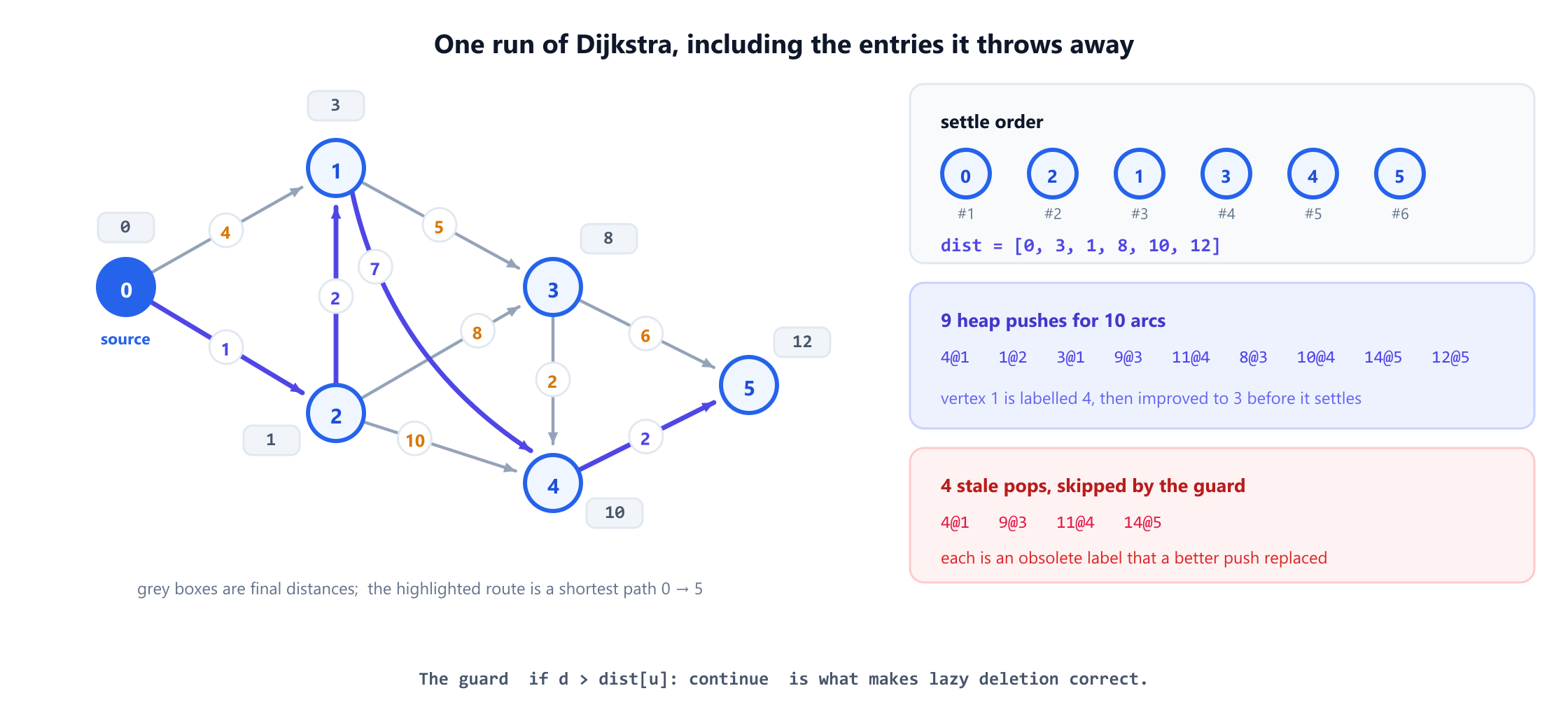
On the running graph Dijkstra from 0 settles in the order 0, 2, 1, 3, 4, 5 and returns distances 0, 3, 1, 8, 10, 12. Watch vertex 1: the arc 0 → 1 labels it 4, then 0 → 2 → 1 improves it to 3 before it is ever popped. That is the algorithm working exactly as intended, and it is why you must not commit to a label at push time.
The follow-up: return the path, not just the length. Keep a parent array, set parent[v] = u in the same branch that improves dist[v], then walk it backwards from the target and reverse. On this graph that gives 0 → 2 → 1 → 4 → 5, cost 12. Say "a shortest path" rather than "the": there are two of cost 12 here, as section 7 shows.
The trap. Setting parent[v] outside the improvement branch, so it records the last vertex that tried rather than the one that succeeded. The distances stay right and the reconstructed path is wrong, which is the worst kind of bug to find in review.
4. Cheapest flights within K stops
The question. Cheapest route from source to target using at most K intermediate stops.
This is the question that catches people, because plain Dijkstra is wrong here. Its correctness rests on a vertex having one final label, but under a stop limit a vertex has a different best cost for each number of stops used, and a cheap route that burns too many hops can be worse than an expensive short one. Settling a vertex once throws away exactly the alternative you need.
Two correct answers, and knowing both is the point.
Widen the state. Keep Dijkstra but make the vertex a pair (node, stops_used). The label is now final per pair, so the invariant holds again.
def cheapest(adj, src, dst, K, n):
    best = [[float('inf')] * (K + 2) for _ in range(n)]
    best[src][0] = 0
    heap = [(0, src, 0)]                     # (cost, node, stops)
    while heap:
        c, u, k = heapq.heappop(heap)
        if u == dst: return c                # first pop of dst is optimal
        if k > K or c > best[u][k]: continue
        for v, w in adj[u]:
            if c + w < best[v][k + 1]:
                best[v][k + 1] = c + w
                heapq.heappush(heap, (c + w, v, k + 1))
    return -1
Or use Bellman-Ford, which is the cleaner answer. Relaxing every edge exactly K + 1 times, each round from a snapshot of the previous round, gives the cheapest route using at most K + 1 edges directly. That is Bellman's 1958 formulation, and it is O(K × E) with no heap at all. Offering it unprompted reads very well.
The trap. The Bellman-Ford version must relax from a copy of the previous round's distances. Relaxing in place lets a single round propagate along several edges, which silently allows more than K stops and returns a too-cheap answer that looks plausible.
5. Path with minimum effort: replacing the plus
The question. Minimise the largest single edge on the route rather than the total. Phrasings: minimum effort path, swim in rising water, the maximum weight you must be able to carry.
The insight is that Dijkstra never actually required addition. It requires that extending a path cannot improve its cost, so that a settled label stays final. max satisfies that just as well as +, so change one line:
        cand = max(d, w)          # instead of d + w
        if cand < best[v]:
            best[v] = cand
            heapq.heappush(heap, (cand, v))
On the running graph the minimax values from vertex 0 are 0, 2, 1, 5, 5, 5, so the best bottleneck to vertex 5 is 5: brute-forcing every route confirms it. That it is a genuinely different objective is visible in the two cheapest routes, which both cost 12 but have largest arcs of 5 and 7. Minimising the total and minimising the largest arc are not the same question, and in general the bottleneck-optimal route need not be a shortest one at all.
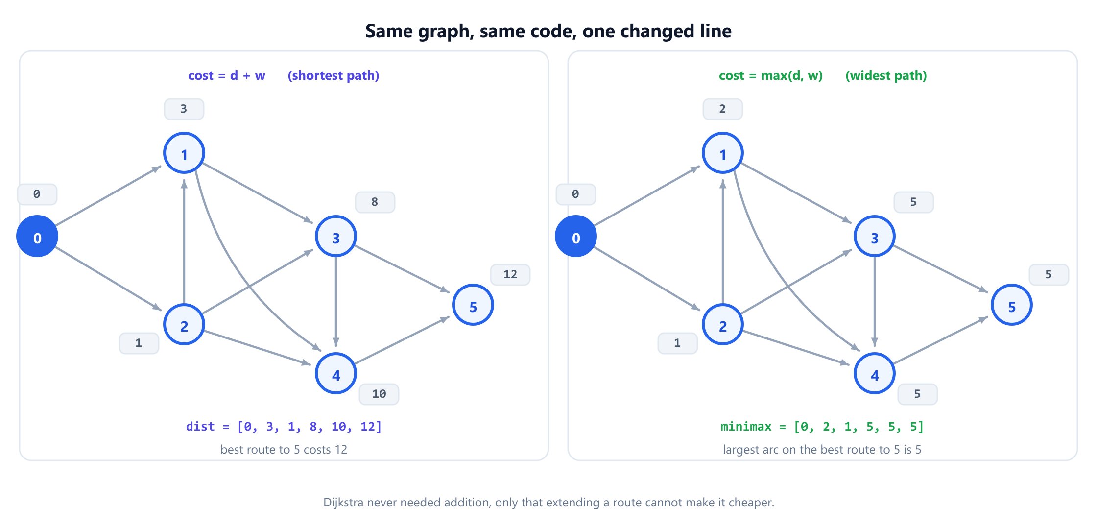
+ for max turns shortest path into widest path.The follow-up: what else can replace the plus? Any operation that is monotone, meaning extending a path never lowers its cost. max works, multiplication by probabilities in [0,1] works if you maximise, and ordinary addition of non-negative weights works. Subtraction does not, which is the same reason negative edges are forbidden.
The trap. On a grid version, a union-find or binary-search-plus-BFS solution is also accepted and is sometimes faster. If you offer Dijkstra, be ready to say why you chose it: no parameter to binary search over, and one pass.
6. Maximum-probability path
The question. Each edge has a success probability; find the route from source to target with the highest probability that every edge succeeds.
Costs multiply rather than add, and you want the largest product, so invert the queue into a max-heap and relax with ×. Probabilities lie in [0,1], so extending a path can only shrink the product, which is exactly the monotonicity Dijkstra needs.
        cand = p * pw                     # instead of d + w
        if cand > best[v]:                # > because we maximise
            best[v] = cand
            heapq.heappush(heap, (-cand, v))   # negate: heapq is a MIN-heap
On a graph with a direct arc of 0.30 from 0 to 3, plus the two-arc route 0 → 1 → 3 at 0.9 and 0.8, the best probability is 0.72 along the two-arc route, beating the single arc. That is the sentence to say: more edges can be better here, which is never true for ordinary shortest paths with positive weights.
The follow-up: why not take logarithms? You can, and it is a good answer. Since log(ab) = log a + log b, maximising a product of probabilities is minimising a sum of -log p, which are non-negative, so unmodified Dijkstra applies. Mention the caveat: floating-point log of a probability near zero loses precision, and an edge of probability 0 gives an infinity you must special-case.
7. Counting shortest paths
The question. How many distinct shortest routes are there from source to target? Usually asked modulo 109+7.
One extra array, and one extra branch. Alongside dist keep ways, the number of shortest routes to each vertex. When a relaxation improves a label, the count is replaced. When it ties, the count is added.
        if d + w < dist[v]:
            dist[v] = d + w
            ways[v] = ways[u]              # strictly better: replace
            heapq.heappush(heap, (dist[v], v))
        elif d + w == dist[v]:
            ways[v] = (ways[v] + ways[u]) % MOD   # a tie: ADD
On the running graph the counts are 1, 1, 1, 1, 2, 2. Brute force agrees: of the 9 routes from 0 to 5, two cost 12, namely 0→2→1→3→4→5 and 0→2→1→4→5. Note the shorter route in edges is not uniquely best, which is the sort of detail worth pointing at.
The follow-up: is the tie branch safe? It is, but only because ways[u] is final when u is popped, and every relaxation happens from a popped vertex. Adding counts from a vertex that has not settled would double count. This is the clearest example of why "settled means final" is the invariant that matters, not the code.
The trap. Forgetting that the elif must sit on the equality, not inside the improvement branch. Written as a single if d + w <= dist[v] the counts are replaced on ties instead of added, and the answer is 1 for every vertex.
8. The second shortest path
The question. Find the second shortest route from source to target. Clarify immediately whether "second" means strictly longer than the best, or simply the next route in a list where ties count separately. The two answers differ and interviewers ask this on purpose.
The technique is to relax the settled-once rule: keep the two best labels per vertex and let a vertex be popped twice.
best1 = [inf] * n; best2 = [inf] * n
best1[src] = 0
heap = [(0, src)]
while heap:
    d, u = heapq.heappop(heap)
    if d > best2[u]: continue          # worse than both labels we keep
    for v, w in adj[u]:
        nd = d + w
        if nd < best1[v]:
            best1[v], nd = nd, best1[v]     # demote the old best to candidate
            heapq.heappush(heap, (best1[v], v))   # the NEW best must propagate too
        if best1[v] < nd < best2[v]:        # strictly worse than best
            best2[v] = nd
            heapq.heappush(heap, (nd, v))
On the running graph the distinct route costs from 0 to 5 are 12, 13, 14, 15, so the strictly-second best is 13. If instead ties count separately, the answer is 12 again, because two different routes achieve it. Ask before you code.
The follow-up: generalise to K. Keep a list of the K best labels per vertex, or use Yen's algorithm for K shortest loopless paths, which is a genuinely different and much heavier problem. Saying "loopless changes it completely" is the right instinct: without that restriction a shortest walk can repeat a zero-weight cycle forever.
9. Why non-negative weights are non-negotiable
Every interviewer asks this, and most candidates answer "because Dijkstra is greedy", which is true and explains nothing. The precise reason: the algorithm assumes that when a vertex is popped with the smallest label in the queue, no route still under construction can reach it more cheaply. A negative edge breaks that, because extending a path can reduce its cost.
Have a concrete counterexample ready. Take four vertices with arcs 0→1 (1), 0→2 (2), 2→1 (−2) and 1→3 (1).
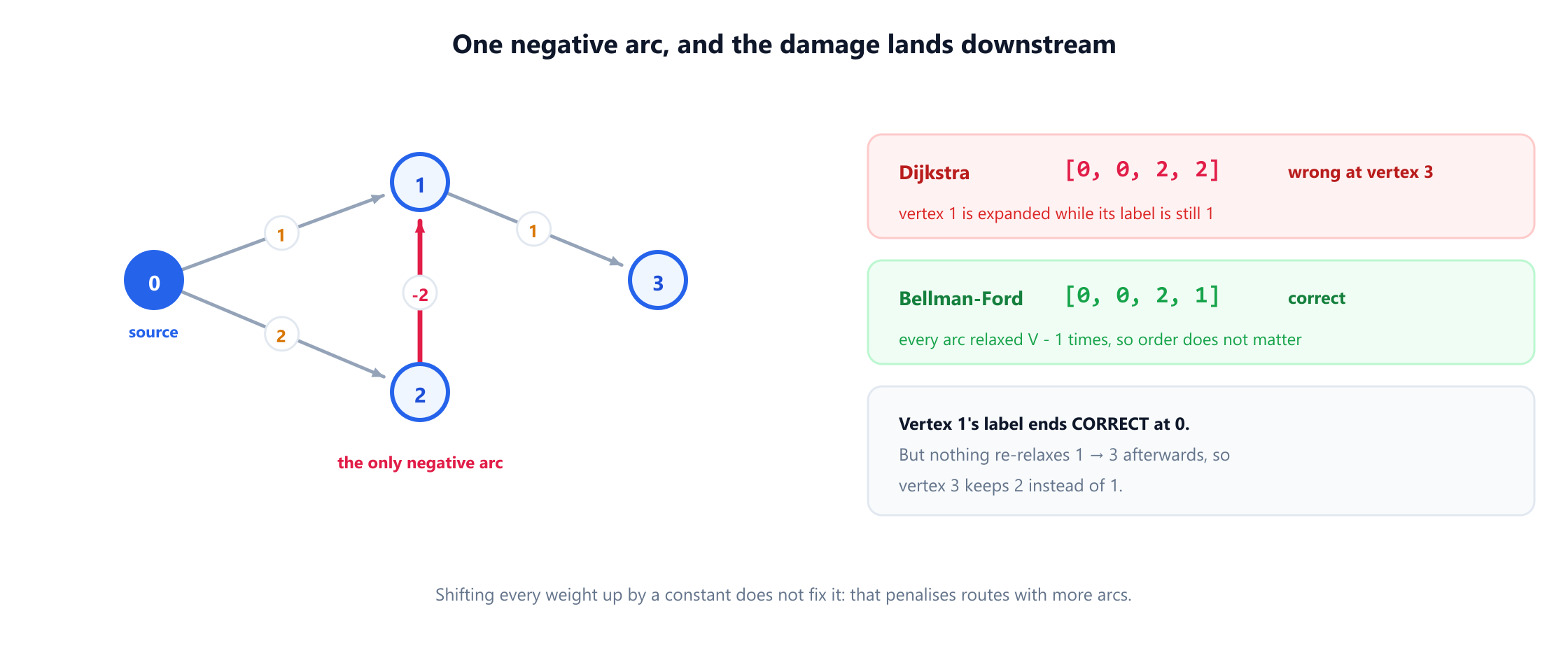
Dijkstra returns 0, 0, 2, 2; the correct answer is 0, 0, 2, 1. The subtlety is worth stating precisely, because it is more interesting than the usual answer: vertex 1's label ends up correct. It is expanded while its label is still 1, and the later improvement to 0 does get written. But nothing re-relaxes 1 → 3 afterwards, so vertex 3 keeps 2 instead of 1. A candidate who says "the wrong value appears downstream of the negative edge, not at it" is clearly speaking from having tried it.
The follow-up: what do you use instead? Bellman-Ford, which relaxes every edge V - 1 times in O(VE) and detects negative cycles on the V-th pass. If you need all pairs and have negative edges but no negative cycle, Johnson's algorithm reweights with one Bellman-Ford run so that every weight becomes non-negative, then runs Dijkstra from each vertex. Cormen, Leiserson, Rivest and Stein give the correctness proof for the greedy choice in full.
The trap. "Just add a constant to every weight to make them positive." It does not work, and being able to say why in one sentence is a strong signal: adding c to every edge adds c × (number of edges) to a route, which penalises routes with more edges, so it changes which route is shortest.
10. The complexity answers
Have the bound and the reason ready, and name the data structure. Saying "Dijkstra is O(E log V)" without naming the heap invites a follow-up you will then fail.
| Priority queue | Time | The reason to give |
|---|---|---|
| Binary heap, lazy deletion | O((V + E) log V) | Up to E entries pushed, each pop and push is logarithmic |
| Fibonacci heap | O(E + V log V) | Decrease-key is O(1) amortised, so edges cost no logarithm |
| Unsorted array | O(V2 + E) | Scan for the minimum each round; best on dense graphs |
| Space, any variant | O(V + E) | The graph, plus a heap that never exceeds E entries |
The heap-based bound is Johnson's 1977 result; the Fibonacci heap improvement is Fredman and Tarjan, 1987. The binary heap itself is Williams' 1964 construction. The Fibonacci variant is theoretically better and almost always slower in practice, because its constants are large, and saying that shows judgement rather than recitation. Sedgewick and Wayne give the shortest clear account of the indexed-priority-queue alternative, which does support decrease-key.
Two numbers worth having. On a sparse graph with V = 105 and E = 5 × 10⁵, the binary-heap bound works out to about 10 million operations against roughly 2.2 million for the Fibonacci heap: a real gap on paper that constants erase in practice. And on a dense graph where E approaches V2, the plain array at O(V2) beats the binary heap's O(V2 log V), which is the one case where the "naive" implementation is the right call.
11. Mistakes that fail the interview
Ordered by frequency; the first three account for most rejected solutions.
- Omitting the stale-entry check. Without
if d > dist[u]: continueyou re-expand vertices from obsolete labels. The answer usually still comes out right, and the running time degrades badly, which is why it survives testing. - Using Dijkstra where the state is not just the vertex. A stop limit, a fuel budget or a "at most K discounts" clause means the label is per
(vertex, resource)pair. Settling the vertex alone discards the route you needed. - Reaching for Dijkstra on negative weights. Use Bellman-Ford, and never try to shift the weights positive.
- Forgetting that
heapqis a min-heap. Maximising anything means pushing the negated key, and forgetting the second negation on the way out is the classic silent bug. - Comparing tuples that contain an unorderable second element.
heappush(heap, (dist, node_object))raises as soon as two distances tie and Python falls through to comparing the objects. Push an index, or add a tiebreaking counter. - Setting the parent pointer outside the improvement branch. Distances stay correct and the reconstructed path is wrong.
- Replacing counts on a tie instead of adding them. One
<=where<and==belonged, and every shortest-path count becomes 1. - Quoting a bound without the data structure. Binary heap, Fibonacci heap and array give three different answers, and the interviewer wants to know you know that.
- Not asking about the input. Directed? Weights non-negative? Can the target be unreachable? Are there parallel edges with different weights? Each changes the code, and Skiena's point holds: problems are won in the modelling.
The habit that prevents most of these: before writing, say what the label means and why extending a route can never improve it. If you cannot say that sentence, the problem is not a Dijkstra problem, and you have just saved yourself twenty minutes. McDowell makes the same argument for interview problems generally.
12. Frequently asked questions
Why can Dijkstra not handle negative weights?
+
Because it assumes that once a vertex is popped with the smallest label in the queue, no route still being built can reach it more cheaply. A negative edge breaks that, since extending a path can reduce its cost. On the four-vertex example with arcs 0 to 1 of weight 1, 0 to 2 of weight 2, 2 to 1 of weight minus 2 and 1 to 3 of weight 1, Dijkstra returns 0, 0, 2, 2 where the truth is 0, 0, 2, 1. Use Bellman-Ford instead.
What is lazy deletion and why do I need it?
+
A binary heap has no efficient decrease-key, so instead of updating a vertex's entry you push a second one with the better label and ignore the obsolete entry when it surfaces. The guard is one line: if the popped distance exceeds the current best for that vertex, skip it. The cost is that the heap can hold up to E entries rather than V, which is why the bound is O((V + E) log V).
Can I use Dijkstra when the path has a limit on the number of edges?
+
Not as written, because a vertex no longer has a single final label: its best cost differs for each number of hops used. Either widen the state so the queue holds pairs of vertex and hops used, which restores the invariant, or use Bellman-Ford and relax every edge exactly K plus one times from a snapshot of the previous round. The second is usually the cleaner answer.
What can I replace the addition with?
+
Anything monotone, meaning extending a route can never lower its cost. Using max instead of plus solves bottleneck or minimum-effort problems. Multiplying probabilities in the range zero to one and maximising works too, and can equivalently be done by minimising the sum of negative logarithms. Subtraction is exactly what fails, which is the same reason negative edges are forbidden.
How do I count the number of shortest paths?
+
Carry a second array holding the number of shortest routes to each vertex. When a relaxation strictly improves a label, replace that count with the predecessor's. When it ties the existing label exactly, add the predecessor's count instead. It is correct only because a vertex's count is final when it is popped, and every relaxation runs from a popped vertex.
Dijkstra or A* in an interview?
+
A* is Dijkstra with a heuristic added to the priority, the 1968 formulation of Hart, Nilsson and Raphael, and it reduces to Dijkstra when that heuristic is zero. Reach for it only when there is a single target and a genuine admissible heuristic, such as straight-line distance on a map or grid. Without one there is nothing to guide the search, and offering A* on an abstract graph signals that you are pattern matching rather than thinking.
Which heap should I say I would use?
+
A binary heap with lazy deletion, giving O((V + E) log V), because it is what every standard library provides and its constants are small. Mention that a Fibonacci heap improves the bound to O(E + V log V) but is slower in practice, and that on a dense graph a plain array scan at O(V squared) beats both. Naming the trade-off matters more than naming the fastest.
13. References
The papers that introduced these techniques and the texts that analyse them, in chronological order.
- Bellman, R. (1958). “On a routing problem.” Quarterly of Applied Mathematics, 16(1), 87–90.
- Dijkstra, E. W. (1959). “A note on two problems in connexion with graphs.” Numerische Mathematik, 1, 269–271.
- Williams, J. W. J. (1964). “Algorithm 232: Heapsort.” Communications of the ACM, 7(6), 347–348.
- Hart, P. E., Nilsson, N. J. and Raphael, B. (1968). “A formal basis for the heuristic determination of minimum cost paths.” IEEE Transactions on Systems Science and Cybernetics, 4(2), 100–107.
- Johnson, D. B. (1977). “Efficient algorithms for shortest paths in sparse networks.” Journal of the ACM, 24(1), 1–13.
- Fredman, M. L. and Tarjan, R. E. (1987). “Fibonacci heaps and their uses in improved network optimization algorithms.” Journal of the ACM, 34(3), 596–615.
- Cormen, T. H., Leiserson, C. E., Rivest, R. L. and Stein, C. (2009). Introduction to Algorithms, 3rd edition, Section 24.3. MIT Press.
- Sedgewick, R. and Wayne, K. (2011). Algorithms, 4th edition, Section 4.4. Addison-Wesley.
- McDowell, G. L. (2015). Cracking the Coding Interview, 6th edition. CareerCup.
- Skiena, S. S. (2020). The Algorithm Design Manual, 3rd edition, Chapter 8. Springer.