
Table of Contents
- 1. What a BFS question is actually testing
- 2. The template to write from memory
- 3. Shortest path in an unweighted graph
- 4. Number of islands
- 5. Rotting oranges: multi-source BFS
- 6. Word ladder: implicit graphs and meeting in the middle
- 7. Level order traversal of a binary tree
- 8. 0-1 BFS: when BFS beats Dijkstra
- 9. Is the graph bipartite?
- 10. Course schedule: BFS topological sort
- 11. The complexity answers interviewers expect
- 12. Mistakes that fail the interview
- 13. Frequently asked questions
- 14. References
1. What a BFS question is actually testing
Almost nobody is asked to "implement BFS". You get a problem that does not look like a graph, and the interview asks three things: can you see the graph, do you know BFS is the tool, and can you write it without a bug.
The signal is the word fewest, or any synonym: minimum steps, shortest transformation, earliest minute, closest exit. BFS answers those, and only when every step costs the same. That clause is the whole game: when steps cost the same BFS gives the exact minimum in O(V + E); when they do not it is simply wrong, and reaching for it is the mistake the question was built around.
The eight below are the ones that recur. Each is presented the way it goes: the problem, the solution, the follow-up the interviewer asks next, and the error that loses the offer. Every worked example was executed by script.
2. The template to write from memory
One template covers every question here. You should be able to produce it in two minutes without thinking, because interview time belongs to the modelling, not the typing.
from collections import deque

def bfs(start, neighbours):
    dist = {start: 0}
    q = deque([start])
    while q:
        u = q.popleft()
        for v in neighbours(u):
            if v not in dist:          # mark ON ENQUEUE, never on dequeue
                dist[v] = dist[u] + 1
                q.append(v)
    return dist
Four details separate a clean pass from a shaky one.
- Mark visited when you enqueue, not when you dequeue. Marking on dequeue lets a vertex be pushed once per incoming frontier edge, blowing the queue up to
O(E). Distances stay correct, so it passes the tests and fails the review. - Use a real queue.
deque.popleft()isO(1);list.pop(0)isO(n)and silently turns a linear algorithm quadratic. - The distance map doubles as the visited set. Two structures where one will do is two chances to forget an update.
neighboursis a function, not a data structure. That is what lets the same eight lines solve a grid, a word puzzle and a state space unmodified. Most interview graphs are never materialised at all, a point developed in graph representation.
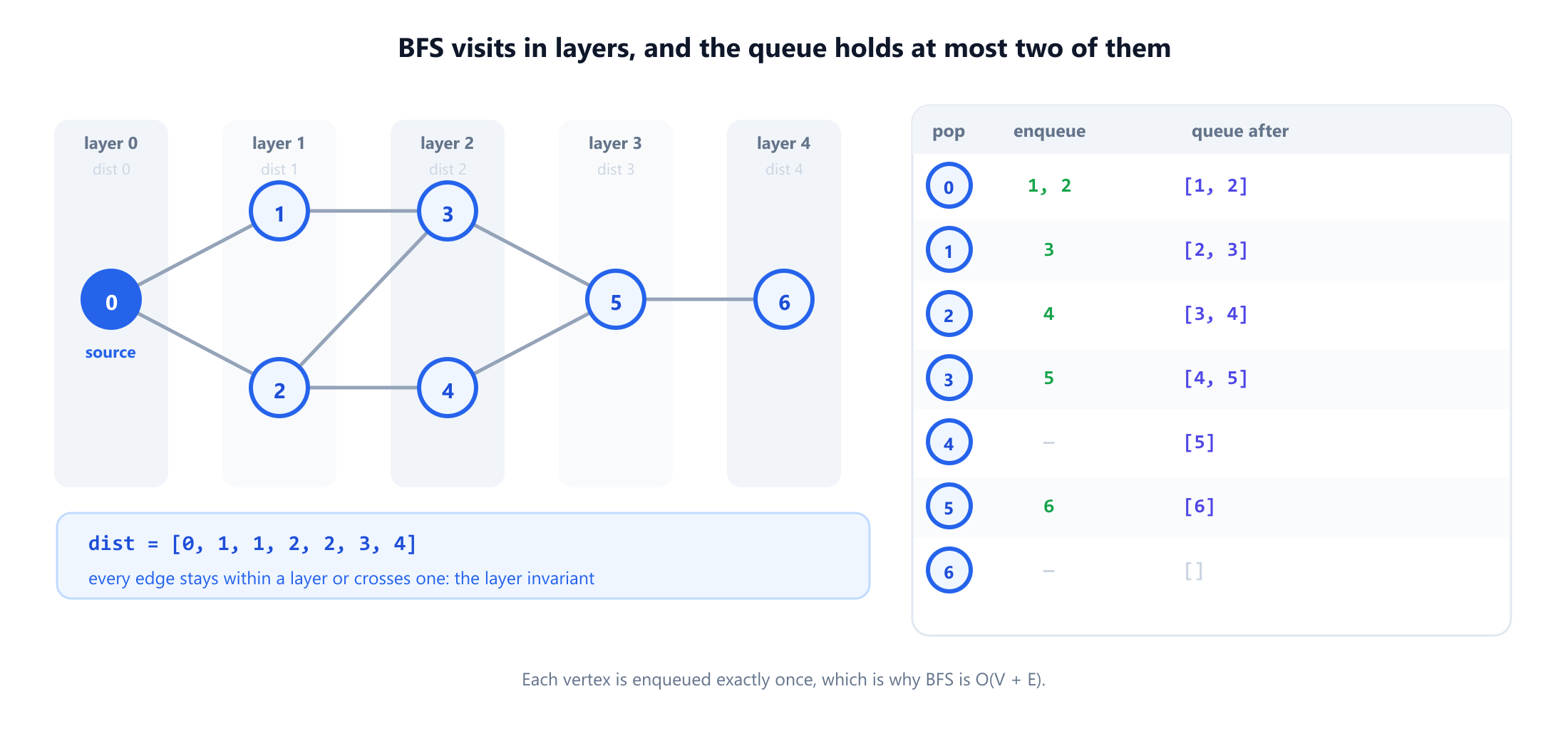
The property that makes this work is the layer invariant: every edge joins vertices in the same layer or in consecutive ones, never skipping. All eight edges above satisfy it, and it is why the first time BFS reaches a vertex is along a shortest path. Say it out loud: "BFS finds the shortest path" without a reason sounds memorised.
3. Shortest path in an unweighted graph
The question. Given an unweighted graph and two vertices, return the shortest path length and the path itself.
The base case. The only addition to the template is a parent pointer.
def shortest_path(adj, src, dst):
    dist, parent = {src: 0}, {src: None}
    q = deque([src])
    while q:
        u = q.popleft()
        if u == dst:                     # early exit: stop when POPPED
            break
        for v in adj[u]:
            if v not in dist:
                dist[v] = dist[u] + 1
                parent[v] = u
                q.append(v)
    if dst not in dist:
        return None
    path, cur = [], dst
    while cur is not None:
        path.append(cur)
        cur = parent[cur]
    return dist[dst], path[::-1]
On the graph in the figure this returns distance 4 and the path 0 → 1 → 3 → 5 → 6. Say unprompted that it is a shortest path, not the one: 0 → 2 → 3 → 5 → 6 is equally short, and which you get depends on adjacency order.
The follow-up: can you exit early? Yes, and the subtlety is where. Testing for the target when you pop is always correct. Testing when you push also works for plain BFS and saves a layer, but stops being correct once weights appear, so the pop-time check is the habit worth having. The worst case is unchanged at O(V + E).
The trap. When the interviewer says "now the edges have weights", do not patch BFS. Switch to Dijkstra's algorithm, or to the deque trick in section 8 if the weights are only 0 and 1. Candidates who make BFS re-visit vertices to cope with weights are writing a slow, buggy Bellman-Ford by accident.
4. Number of islands
The question. Given a grid of '1' (land) and '0' (water), count the connected groups of land. Diagonals do not connect.
There is no explicit graph, which is the point. Vertices are land cells, edges are shared sides, so a cell has at most four neighbours and you never build an adjacency structure.
def num_islands(grid):
    if not grid: return 0
    R, C = len(grid), len(grid[0])
    seen, count = set(), 0
    for i in range(R):
        for j in range(C):
            if grid[i][j] != '1' or (i, j) in seen:
                continue
            count += 1
            seen.add((i, j))
            q = deque([(i, j)])
            while q:
                r, c = q.popleft()
                for dr, dc in ((1,0), (-1,0), (0,1), (0,-1)):
                    a, b = r + dr, c + dc
                    if 0 <= a < R and 0 <= b < C \
                       and grid[a][b] == '1' and (a, b) not in seen:
                        seen.add((a, b))
                        q.append((a, b))
    return count
Every cell is enqueued at most once and each does constant work, so this is O(R × C) time. Space is the visited set plus the queue, also O(R × C) in the worst case, when the grid is entirely land.
The follow-up: BFS or DFS? Either works, because you are labelling components rather than measuring distance. Prefer BFS for a practical reason: recursive DFS on a 106-cell grid of solid land recurses a million deep and overflows the stack. If you pick DFS, say you would write it iteratively; that sentence is often the whole point of the follow-up. The comparison is in BFS vs DFS.
The trap. Mutating the input grid, writing '0' over land instead of keeping a visited set, is a legitimate optimisation, but say that you are doing it. Silently destroying the caller's data is a code-review failure, not a cleverness.
5. Rotting oranges: multi-source BFS
The question. A grid holds empty cells (0), fresh oranges (1) and rotten ones (2). Each minute, every rotten orange rots the fresh oranges orthogonally adjacent to it. Return the number of minutes until none are fresh, or -1 if that never happens.
This separates people who memorised BFS from people who understand it. The instinct is to run a BFS from each rotten orange and combine the results, which is complicated and slow. The answer is to put every rotten orange in the queue before the loop starts. BFS then expands one shared wavefront, and each cell is reached first by whichever source is nearest.
def oranges_rotting(grid):
    R, C = len(grid), len(grid[0])
    q, fresh = deque(), 0
    for i in range(R):
        for j in range(C):
            if grid[i][j] == 2: q.append((i, j, 0))
            elif grid[i][j] == 1: fresh += 1

    minutes = 0
    while q:
        r, c, t = q.popleft()
        minutes = max(minutes, t)
        for dr, dc in ((1,0), (-1,0), (0,1), (0,-1)):
            a, b = r + dr, c + dc
            if 0 <= a < R and 0 <= b < C and grid[a][b] == 1:
                grid[a][b] = 2                  # mark on enqueue
                fresh -= 1
                q.append((a, b, t + 1))
    return -1 if fresh else minutes
Worked on this grid:
2 1 1 0          minute each cell rots:      0  1  2  .
1 1 0 2                                      1  2  .  0
0 1 1 1                                      .  3  2  1

two sources, 7 fresh oranges, 0 remaining, answer = 3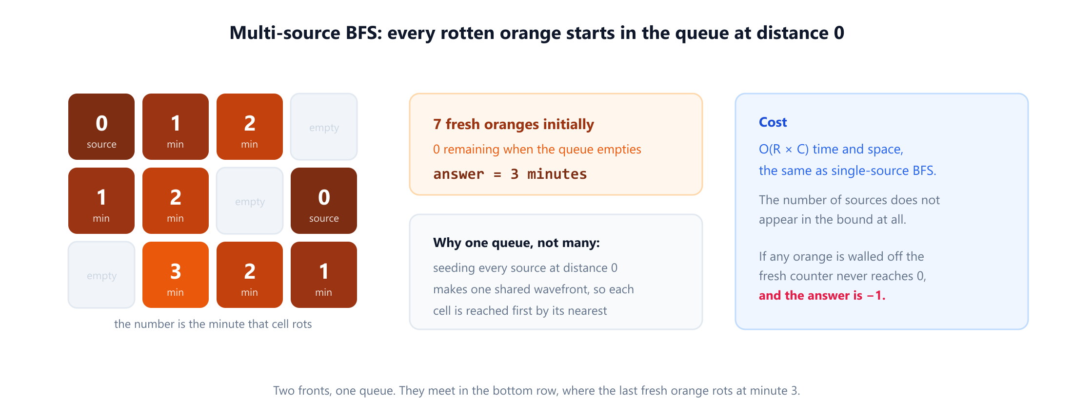
Complexity is O(R × C), unchanged by the number of sources. That multi-source BFS costs the same as single-source BFS is the insight being tested.
The follow-up: what if an orange can never rot? That is the -1 case, and why the fresh counter exists. Do not detect it by comparing visited cells against the grid size: empty cells are not oranges and the arithmetic goes wrong. Count fresh up front, decrement on each rot, check what remains. Empty the two cells beside the bottom-left orange and it is sealed off, so one stays fresh and the answer is -1.
The trap. The empty grid. Zero fresh and zero rotten should return 0, and an off-by-one returning 1 is the most common wrong submission.
6. Word ladder: implicit graphs and meeting in the middle
The question. Given a start word, an end word and a dictionary, find the length of the shortest chain where each step changes exactly one letter and every intermediate word is in the dictionary.
The graph has one vertex per dictionary word and an edge between words differing in one position. Building it explicitly costs O(N2 L) time, which is the slow solution most candidates write first. The fast one never builds it: generate neighbours on demand by trying all 26 letters at each of the L positions and testing against a hash set, exactly as the code below does. One substitution per position regenerates the word itself and the visited check discards it. For ten-letter words that is 260 lookups per vertex, independent of dictionary size.
def ladder_length(begin, end, word_list):
    words = set(word_list)
    if end not in words: return 0
    q, dist = deque([begin]), {begin: 1}
    while q:
        w = q.popleft()
        if w == end: return dist[w]
        for i in range(len(w)):
            for ch in "abcdefghijklmnopqrstuvwxyz":
                nxt = w[:i] + ch + w[i+1:]
                if nxt in words and nxt not in dist:
                    dist[nxt] = dist[w] + 1
                    q.append(nxt)
    return 0
The follow-up: make it faster. The expected answer is bidirectional BFS, introduced by Pohl in 1971: search forward from the start and backward from the end at once, always expanding the smaller frontier, and stop when they meet. A one-directional search to depth d with branching factor b touches about bd vertices; two searches of depth d/2 touch 2bd/2. That is a halving of the exponent, not a constant factor.
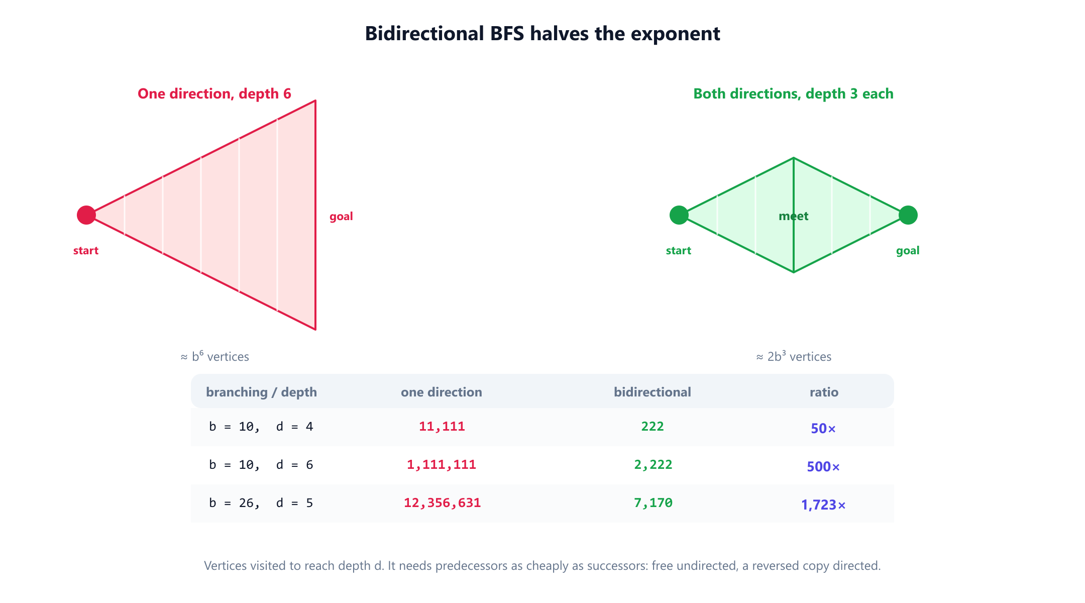
The deeper the answer lies, the more this buys.
The trap. Bidirectional BFS needs predecessors as cheaply as successors: free here, since the relation is symmetric, but a reversed copy on a directed graph. The meeting point also needs care. The answer is the sum of the two depths, and stopping the instant a vertex appears in both visited sets is only valid when you expand a whole layer at a time.
7. Level order traversal of a binary tree
The question. Return the values of a binary tree grouped by depth, one list per level.
The only new idea is processing a whole layer at a time, and the trick is to record the queue's length before the inner loop.
def level_order(root):
    if not root: return []
    out, q = [], deque([root])
    while q:
        level = []
        for _ in range(len(q)):        # snapshot the layer size FIRST
            node = q.popleft()
            level.append(node.val)
            if node.left:  q.append(node.left)
            if node.right: q.append(node.right)
        out.append(level)
    return out
Capturing len(q) in the range call is what makes this work: the loop runs exactly as many times as there were nodes on the level, even though the queue grows during it. Reading the length inside the loop silently merges levels, and is the classic bug here.
A tree needs no visited set: no cycles, one parent per node. Say that you are dropping it because the input is a tree, since dropping it silently on a graph is a hang.
The follow-ups. Zigzag order reverses level on odd depths, rather than queueing backwards. Right side view is the last element of each level. Minimum depth is the depth of the first leaf popped, and here BFS genuinely beats DFS, which must explore the whole tree.
8. 0-1 BFS: when BFS beats Dijkstra
The question. Every edge has weight 0 or 1; find the shortest distance from a source. Variants appear as a grid where some moves are free, or as "minimum walls to break".
Dijkstra solves this in O(E log V) and is accepted. The answer being fished for runs in O(V + E): use a double-ended queue, pushing a relaxed vertex to the front across a 0-weight edge and the back across a 1-weight edge. The deque then holds at most two distinct distance values at once, which is exactly the ordering a priority queue was providing.
def zero_one_bfs(adj, src, n):        # adj[u] = [(v, w), ...] with w in {0, 1}
    dist = [float('inf')] * n
    dist[src] = 0
    dq = deque([src])
    while dq:
        u = dq.popleft()
        for v, w in adj[u]:
            if dist[u] + w < dist[v]:
                dist[v] = dist[u] + w
                if w == 0: dq.appendleft(v)
                else:      dq.append(v)
    return dist
On a graph with edges 0-1 (weight 1), 0-2 (0), 2-3 (1), 1-3 (0), 3-4 (1) and 2-4 (1), this returns 0, 1, 0, 1, 1, matching Dijkstra exactly. Plain BFS returns 0, 1, 1, 2, 2, wrong for three of the five vertices, because it counts edges instead of summing weights. That contrast is the cleanest way to show what BFS actually optimises.
The technique belongs to the label-correcting family, whose general form Bertsekas set out in 1993. One structural difference from ordinary BFS matters: a vertex can be relaxed more than once, so the guard is a distance comparison, not a visited check.
The trap. Writing if v not in visited instead of if dist[u] + w < dist[v]. The visited check lets the first arrival win, and across a 0-weight edge the first arrival need not be the best. The code still runs and returns plausible numbers.
9. Is the graph bipartite?
The question. Can the vertices be split into two sets so that every edge crosses between them? Phrased in interviews as "split these people so no two enemies share a group", or "is this graph 2-colourable".
Colour the source 0, colour every neighbour with the opposite colour, and fail if you ever meet a neighbour already carrying your own colour.
def is_bipartite(adj, n):
    colour = [-1] * n
    for s in range(n):
        if colour[s] != -1: continue      # a new component
        colour[s] = 0
        q = deque([s])
        while q:
            u = q.popleft()
            for v in adj[u]:
                if colour[v] == -1:
                    colour[v] = 1 - colour[u]
                    q.append(v)
                elif colour[v] == colour[u]:
                    return False
    return True
The clean explanation: the colour is the parity of the BFS layer. A conflict means an edge joins two vertices in the same layer, closing a cycle of odd length, and a graph is bipartite exactly when it has no odd cycle. The 4-cycle is bipartite, the 5-cycle is not, and the algorithm confirms both.
The trap, and it fails more submissions than any other: the outer for s in range(n) loop. A disconnected graph needs BFS restarted from every uncoloured vertex, so a solution starting only at vertex 0 passes every connected test and fails the moment there are two components. Counting components and detecting cycles need the same loop.
10. Course schedule: BFS topological sort
The question. Given n courses and a list of prerequisite pairs, can every course be taken? The follow-up asks for a valid order.
This is cycle detection on a directed graph, and the BFS answer is Kahn's algorithm (1962): repeatedly take a vertex with no remaining prerequisites, remove it, decrement its successors.
def find_order(n, prerequisites):
    adj = [[] for _ in range(n)]
    indeg = [0] * n
    for course, prereq in prerequisites:
        adj[prereq].append(course)
        indeg[course] += 1

    q = deque(i for i in range(n) if indeg[i] == 0)
    order = []
    while q:
        u = q.popleft()
        order.append(u)
        for v in adj[u]:
            indeg[v] -= 1
            if indeg[v] == 0:
                q.append(v)
    return order if len(order) == n else []    # short == cycle
With 6 courses and prerequisites 1←0, 2←0, 3←1, 3←2, 4←3, 5←4 this schedules all six as 0, 1, 2, 3, 4, 5. With the cyclic set 1←0, 2←1, 0←2 it schedules none: every vertex starts with in-degree 1, so the initial queue is empty. One test covers both cases, and it is the heart of the answer: if the output is shorter than n, the leftover vertices form a cycle.
The trap. Getting the edge direction backwards. The pair [a, b] means "to take a, first take b", so the edge runs b → a and it is a's in-degree that rises. Reverse it and you get a valid topological order of the reversed graph: it looks right, passes the cycle check, and is wrong. Read the direction out loud before writing the loop. Broader treatment in topological sorting.
The depth-first counterpart, covering cycle detection, topological sort, strongly connected components and bridges, is in DFS interview questions.
11. The complexity answers interviewers expect
Half of a BFS interview is analysis. What to say, and why:
| Problem shape | Time | Space | The reason to give |
|---|---|---|---|
| Graph, adjacency list | O(V + E) | O(V) | Each vertex is enqueued once, each edge examined twice |
| Graph, adjacency matrix | O(V2) | O(V) | Finding one vertex's neighbours scans a whole row |
Grid, R × C | O(R × C) | O(R × C) | V = RC and E < 2RC, so V + E is linear in cells |
| Multi-source grid | O(R × C) | O(R × C) | Unchanged: sources only seed the same single wavefront |
Word ladder, N words of length L | O(N × L2 × 26) | O(N × L) | 26L candidates per word, each O(L) to build and hash |
Bidirectional, branching b, depth d | O(bd/2) | O(bd/2) | Two half-depth searches, so the exponent halves |
| 0-1 BFS | O(V + E) | O(V) | A deque replaces the heap, so no log factor |
Two points reward volunteering. The O(V) space is not incidental: BFS holds a whole layer, which on a wide graph is most of the vertex set. That is the real reason to prefer DFS on deep, narrow graphs, and a better answer than "DFS uses less memory", which is not always true. And the edge term is E directed but 2E undirected. Cormen, Leiserson, Rivest and Stein give the full analysis; Sedgewick and Wayne the clearest short one.
BFS was published twice before it had a name: Moore in 1959 for the shortest path through a maze, Lee in 1961 for routing circuit boards. Lee's version is literally the grid BFS of sections 4 and 5, which is why grid pathfinding is still sometimes called Lee's algorithm.
Once the edges carry different weights the queue becomes a priority queue; those problems are worked through in Dijkstra interview questions.
12. Mistakes that fail the interview
Ordered by frequency, not severity. The first three account for most rejected solutions.
- Marking visited on dequeue instead of enqueue. Distances stay correct so tests pass, but the queue grows to
O(E), which on a dense graph is the difference between passing and timing out. - Using a list as a queue.
list.pop(0)and JavaScript'sshift()areO(n). Usecollections.deque, or an index pointer into an array in a language without one. - Forgetting the outer loop over components. Bipartite checking, component counting and cycle detection all restart BFS from every unvisited vertex. Starting only at vertex 0 passes every connected test and fails the first disconnected one.
- Reaching for BFS on a weighted graph. BFS minimises the number of edges, not total weight. If two edges differ in cost you need Dijkstra, or 0-1 BFS when the weights are only 0 and 1.
- Reading the queue length inside the layer loop. In level order traversal,
for _ in range(len(q))must snapshot the length before the loop, or levels merge. - Not asking about the input. Directed? Connected? Self-loops or parallel edges? Are grid diagonals neighbours? Can the start equal the goal? Each changes the code, and Skiena's point holds: problems are won in the modelling, not the traversal.
- Announcing
O(V + E)without saying which representation. The bound belongs to the adjacency list. On a matrix the same code isO(V2).
One habit beats all of the above. Before writing code, say out loud what the vertices are, what the edges are, and what a step costs. If every step costs the same, BFS is correct; if not, you have avoided the trap. McDowell makes the same point generally, and it bites hardest on graphs, where the graph is so often hidden.
13. Frequently asked questions
How do I know a problem wants BFS and not DFS?
+
Look for the word fewest, or a synonym: minimum steps, shortest transformation, earliest minute, nearest exit. BFS answers those exactly, provided every step costs the same. If the question only asks about reachability or connected components, either traversal works, and BFS avoids deep recursion on large inputs.
Why must I mark a vertex visited when I enqueue it?
+
Because between being enqueued and dequeued, a vertex can be discovered again by others in the same frontier. Marking on dequeue lets it be pushed once per incoming edge, so the queue holds O(E) entries instead of O(V). The distances still come out right, which is what makes the bug easy to miss.
What is multi-source BFS and when do I need it?
+
You push every source into the queue before the loop starts, all at distance zero. BFS expands one shared wavefront, so each cell is reached first by whichever source is nearest. It costs the same as single-source BFS, O(V + E). Rotting oranges and nearest-exit problems are the standard examples.
Can BFS ever handle weighted edges?
+
Only when every weight is 0 or 1. Then a double-ended queue, pushing to the front across a zero-weight edge and the back across a one-weight edge, gives the right answer in O(V + E) with no logarithmic factor. For any other weights BFS is simply wrong, because it minimises the number of edges rather than the total weight, and you need Dijkstra.
How much faster is bidirectional BFS?
+
It halves the exponent rather than dividing by a constant, turning roughly b to the power d into 2 times b to the power d over 2. At branching factor 10 and depth 6 that is 1,111,111 vertices against about 2,222, a factor of 500. It needs predecessors to be as cheap as successors: free undirected, a reversed copy directed.
What complexity should I state for a grid BFS?
+
O(R times C) for both time and space. The reason to give is that the grid is a graph with R times C vertices and fewer than 2 R C edges, so V plus E is linear in the cell count. The space is the visited set plus the queue, which can hold a large fraction of the grid at once.
Do I need a visited set when running BFS on a tree?
+
No. A tree has no cycles and every node has one parent, so no node is reached twice and the set would never reject anything. Say why you are omitting it rather than omitting it silently: the same omission on a general graph is an infinite loop, and the interviewer cannot tell which you meant.
14. References
The papers that introduced these techniques and the texts that analyse them, in chronological order.
- Moore, E. F. (1959). “The shortest path through a maze.” Proceedings of an International Symposium on the Theory of Switching, Harvard University Press, 285–292.
- Lee, C. Y. (1961). “An algorithm for path connections and its applications.” IRE Transactions on Electronic Computers, EC-10(3), 346–365.
- Kahn, A. B. (1962). “Topological sorting of large networks.” Communications of the ACM, 5(11), 558–562.
- Pohl, I. (1971). “Bi-directional search.” In Machine Intelligence 6, Edinburgh University Press, 127–140.
- Bertsekas, D. P. (1993). “A simple and fast label correcting algorithm for shortest paths.” Networks, 23(8), 703–709.
- Cormen, T. H., Leiserson, C. E., Rivest, R. L. and Stein, C. (2009). Introduction to Algorithms, 3rd edition, Section 22.2. MIT Press.
- Sedgewick, R. and Wayne, K. (2011). Algorithms, 4th edition, Section 4.1. Addison-Wesley.
- McDowell, G. L. (2015). Cracking the Coding Interview, 6th edition. CareerCup.
- Skiena, S. S. (2020). The Algorithm Design Manual, 3rd edition, Chapter 5. Springer.